felixity-the-cat / Unsupervised-Trajectory-Clustering-Starter

Unsupervised Trajectory Clustering: Getting Started

The code uses mixtures of state space models to perform unsupervised clustering of short trajectories. Within the state space framework, we let expensive-to-gather biomarkers correspond to hidden states and readily obtainable cognitive metrics correspond to measurements. Upon training with expectation maximization, we often find that our clusters stratify persons according to clinical outcome. Furthermore, we can effectively predict on held-out trajectories using cognitive metrics alone. Our approach accommodates missing data through model marginalization and generalizes across research and clinical cohorts.

Data format

We consider a training dataset

$$ \mathcal{D} = { (x_{1:T}^{i}, z_{1:T}^{i}) }_{1\leq i \leq n_d} $$

consisting of $n_d$ sequences of states and observations paired in time. We denote the states $z_{1:T}^{i} = (z_1^i, z_2^i, \dotsc, z_T^i)$ where $z_t^i \in \mathbb{R}^d$ corresponds to the state at time $t$ for the $i$ th instance and measurements $x_{1:T}^{i} = (x_1^i, x_2^i, \dotsc, x_T^i)$ where $x_t^i \in \mathbb{R}^\ell$ corresponds to the observation at time $t$ for the $i$ th instance. For the purposes of this code, we adopt the convention that collections of time-delineated sequences of vectors will be stored as 3-tensors, where the first dimension spans time $1\leq t \leq T$, the second dimension spans instances $1\leq i \leq n_d$ (these will almost always correspond to an individual or participant), and the third dimension spans the components of each state or observation vector (and so will have dimension either $d$ or $\ell$). We accommodate trajectories of differing lengths by standardising to the longest available trajectory in a dataset and appending np.nan's to shorter trajectories.

Model specification

We adopt a mixture of state space models for the data:

$$ p(z^i_{1:T}, x^i_{1:T}) = \sum_{c=1}^{n_c} \pi_{c} \delta_{ \{c=c^i \} } \bigg( p(z_1^i| c) \prod_{t=2}^T p(z_t^i | z_{t-1}^i, c) \prod_{t=1}^T p(x_t^i | z_t^i, c) \bigg) $$

Each individual $i$ is independently assigned to some cluster $c^i$ with probability $\pi_{c}$, and then conditional on this cluster assignment, their initial state $z_1^i$ is drawn according to $p(z_1^i| c)$, with each subsequent state $z_t^i, 2\leq t \leq T$ being drawn in turn using the cluster-specific state model $p(z_t^i | z_{t-1}^i, c)$, depending on the previous state. At each point in time, we obtain an observation $x_t^i$ from the cluster-specific measurement model $p(x_t^i | z_t^i, c)$, depending on the current state. In what follows, we assume both the state and measurement models are stationary for each cluster, i.e. they are independent of $t$. In particular, for a given individual, the relationship between the state and measurement should not change over time.

In our main framework, we additionally assume that the cluster-specific state initialisation is Gaussian, i.e. $p(z_1^i| c) = \eta_d(z_1^i; m_c, S_c)$, and the cluster-specific state and measurement models are linear Gaussian, i.e. $p(z_t^i | z_{t-1}^i, c) = \eta_d(z_t^i; z_{t-1}^iA_c, \Gamma_c)$ and $p(x_t^i | z_t^i, c) = \eta_\ell(x_t^i; z_t^iH_c, \Lambda_c)$, where $\eta_d(\cdot, \mu, \Sigma)$ denotes the multivariate $d$-dimensional Gaussian density with mean $\mu$ and covariance $\Sigma$, yielding:

$$ p(z^i_{1:T}, x^i_{1:T}) = \sum_{c=1}^{n_c} \pi_{c} \delta_{ \{c=c^i \} } \big( \eta_d(z_1^i; m_c, S_c) \prod_{t=2}^T \eta_d(z_t^i; z_{t-1}^iA_c, \Gamma_c) \prod_{t=1}^T \eta_\ell(x_t^i; z_t^iH_c, \Lambda_c) \big). $$

In particular, we assume that the variables we are modeling are continuous and changing over time. When we train a model like the above, we take a dataset $\mathcal{D}$ and an arbitrary set of cluster assignments $c^i$ (as these are also latent/ hidden from us) and iteratively perform M and E steps (from which EM¹ gets its name):

• (E) Expectation step: given the current model, we assign each data instance $(z^i_{1:T}, x^i_{1:T})$ to the cluster to which it is mostly likely to belong under the current model
• (M) Maximization step: given the current cluster assignments, we compute the sample-level cluster assignment probabilities (the $\pi_c$) and optimal cluster-specific parameters

Optimization completes after a fixed (large) number of steps or when no data instances change their cluster assignment at a given iteration.

To run the code

All model training and predictions are done in Python. We provide a pip-installable package unsupervised-multimodal-trajectory-modeling to do much of the work for you. It can be installed with dependencies as follows:

pip3 install -r requirements.txt

or in a virtual environment with:

python3 -m venv venv
source venv/bin/activate
pip3 install -r requirements.txt

Adapting the code for your own use

A typical workflow for a new dataset looks like this:

1. Create a new data_*.py file that organises the data into tensors of states and measurements as described above. Often, we include functionality for plotting trajectories of states by inferred cluster here. This is also a useful place to wrangle auxiliary data that will then be used to profile learned clusters. For example data_synthetic.py, gives us trajectories in state space that look like this: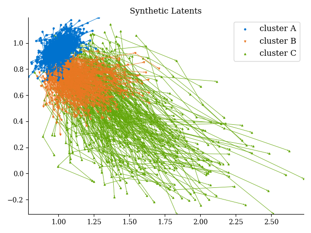

   

2. Run a model selection script to create plots of BIC vs. number of clusters. Import the data_*.py file you created in the previous step and modify model_selection_synthetic.py as needed. This will give us a plot like so: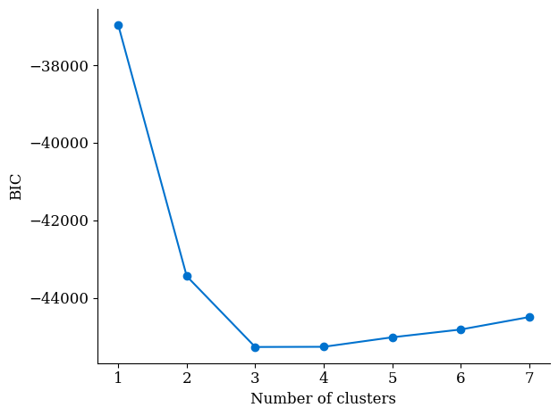

   

   We know the data was generated from a 3-component mixture model, and the BIC plot above reflects that. We now focus on models with 3 clusters.

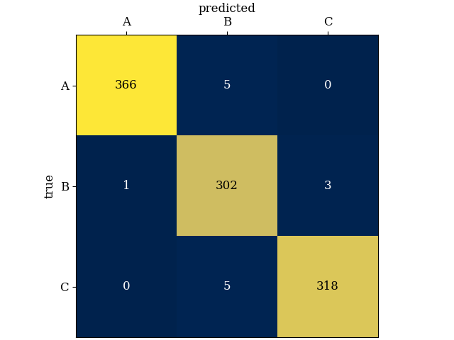
3. Experiment with training and testing, like in inference_synthetic.py. We can, for example, train a model on one set and then predict cluster membership for a new dataset. When both datasets were generated according to the same specifications, we find very good agreement for this example, even when predictions are made without access to the states. Here's a confusion matrix (having generated the test set, we know ground truth):

   

   For real-life examples, we are often interested in profiling our clusters to better understand them.

4. We have an extended framework to incorporate nonlinearities into our state and measurement models. Check out inference_nonlinear.py for a minimal example.

Caveats

Some efforts have been made to handle edge cases. For a given training run, if any cluster becomes too small, training automatically terminates.

Footnotes

1. A. Dempster, N. Laird, and D. B. Rubin. Maximum Likelihood from
   Incomplete Data via the EM Algorithm. J. Roy. Stat. Soc. Ser. B (Stat. Methodol.) 39.1 (1977), pp. 1–38. ↩