
In case you have any question or suggestion, please get in touch sending us an e-mail in felipemaiapolo@gmail.com.
- Introduction
- Installing InfoSelect
- Main functionalities of InfoSelect
- Examples of InfoSelect use
- References
In this package we implement the ideas proposed by [1, 2] in order to make variable/feature selection prior to regression and classification tasks using Gaussian Mixture Models (GMMs) to estimate the Mutual Information between labels and features. This is an efficient and well-performing alternative and was used in a recent work [3] by one of us:
@article{maia2022effective,
  title={Effective sample size, dimensionality, and generalization in covariate shift adaptation},
  author={Maia Polo, Felipe and Vicente, Renato},
  journal={Neural Computing and Applications},
  pages={1--13},
  year={2022},
  publisher={Springer}
}


@misc{polo2020infoselect,
  title={InfoSelect - Mutual Information Based Feature Selection in Python},
  author={Polo, Felipe Maia and Da Silva, Felipe Leno},
  journal={GitHub: github.com/felipemaiapolo/infoselect},
  year={2020}
}
You can install the package from PyPI
$ pip install infoselect
Also, you can install the package from GitHub.
$ pip install git+https://github.com/felipemaiapolo/infoselect.git#egg=infoselect
This class is used to order features/variables according to their importance and making the selection itself. Next we detail its methods:
-
__init__(self, gmm, selection_mode = 'forward')- gmm:
- If
is non-categorical: a Scikit-Learn GMM fitted in (y,X) - y should always be in the first column;
- If
{0:gmm0, 1:gmm1, ..., C:gmmC}; - Please use auxiliary function
get_gmmbelow, especially if you want to usecovariance_typeother than 'full'.
- If
- selection_mode:
forward/backwardalgorithms.forwardselection: we start with an empty set of features and then select the feature that has the largest estimated mutual information with the target variable and. At each subsequent step, we select the feature that marginally maximizes the estimated mutual information of the target and all the chosen features so far. We stop when we have selected/ordered all the features;backwardelimination: we start with the full set of features and then at each step, we eliminate the feature that marginally maximizes the estimated mutual information of the target and all the remaining features. We stop when we have no more features to eliminate;
- gmm:
-
fit(self, X, y, verbose=True, eps=0)- X: numpy array of features;
- y: numpy array of labels;
- verbose: print or not to print!?
- eps: small value so we can avoid taking log of zero in some cases .
-
get_info(self):- This function creates and outputs a Pandas DataFrame with the history of feature selection/elimination. The
mi_meancolumn gives the estimated Mutual Information whilemi_errorgives the standard error of that estimate. On the other hand, thedeltacolumn gives us the percentual information loss/gain in that round, relatively to the latter;
- This function creates and outputs a Pandas DataFrame with the history of feature selection/elimination. The
-
plot_delta(self):- This function plots the history of percentual changes in the mutual information.
-
plot_mi(self):- This function plots the history of the mutual information.
-
transform(self, X, rd):- This function takes X and transforms it in X_new, maintaining the features of Round
rd;
- This function takes X and transforms it in X_new, maintaining the features of Round
-
get_gmm(X, y, y_cat=False, num_comps=[2,5,10,15,20,30,40,50], val_size=0.33, reg_covar=1e-06, covariance_type="full", random_state=42):-
Firstly, this function validate the number of GMM components, for each model it will train, in a holdout set using the mean log likelihood of samples in that set. If Y is non-categorical, it returns a Scikit-Learn GMM fitted in (y,X) model (in this order). On the other hand, if Y is categorical it returns a Python dictionary containing one Scikit-Learn GMM fitted in X conditional on each category - something like X[y==c,:]. Format
{0:gmm0, 1:gmm1, ..., C:gmmC}.- X: numpy array of features;
- y: numpy array of labels;
- y_cat: if we should consider Y as categorical;
- num_comps: numbers of GMM components to be validated;
- val_size: size of holdout set used to validate the GMMs numbers of components;
- reg_covar: non-negative regularization added to the diagonal of covariance. Ensures the covariance matrices are non-singular.
- covariance_type: one of the following options:'full','tied','diag','spherical'. See Scikit-Learn GMM. Thanks to Pritha Gupta for her suggestion on this point.
- random_state: seed.
-
Loading Packages:
import infoselect as inf
import numpy as np
import pandas as pd
import matplotlib.pyplot as pltWe generate a dataset sampled from
similar to the one in here, in which
is given by
Where and
independent from all the other random variables for all
. See that our target variable does not depende on the last two features. In the following we set
n=10000:
def f(X,e): return 10*np.sin(np.pi*X[:,0]*X[:,1]) + 20*(X[:,2]-.5)**2 + 10*X[:,3] + 5*X[:,4] + en=10000
d=7
X = np.random.uniform(0,1,d*n).reshape((n,d))
e = np.random.normal(0,1,n)
y = f(X,e)
X.shape, y.shape((10000, 7), (10000,))
Training (and validating) GMM:
%%time

gmm = inf.get_gmm(X, y)
Wall time: 8.43 s
Ordering features by their importances using the Backward Elimination algorithm:
select = inf.SelectVars(gmm, selection_mode = 'backward')
select.fit(X, y, verbose=True)
Let's start...
Round = 0 | Î = 1.36 | Δ%Î = 0.00 | Features=[0, 1, 2, 3, 4, 5, 6]
Round = 1 | Î = 1.36 | Δ%Î = -0.00 | Features=[0, 1, 2, 3, 4, 5]
Round = 2 | Î = 1.36 | Δ%Î = -0.00 | Features=[0, 1, 2, 3, 4]
Round = 3 | Î = 0.97 | Δ%Î = -0.29 | Features=[0, 1, 3, 4]
Round = 4 | Î = 0.73 | Δ%Î = -0.24 | Features=[0, 1, 3]
Round = 5 | Î = 0.40 | Δ%Î = -0.46 | Features=[0, 3]
Round = 6 | Î = 0.21 | Δ%Î = -0.48 | Features=[3]
Checking history:
select.get_info()| rounds | mi_mean | mi_error | delta | num_feat | features | |
|---|---|---|---|---|---|---|
| 0 | 0 | 1.358832 | 0.008771 | 0.000000 | 7 | [0, 1, 2, 3, 4, 5, 6] |
| 1 | 1 | 1.358090 | 0.008757 | -0.000546 | 6 | [0, 1, 2, 3, 4, 5] |
| 2 | 2 | 1.356661 | 0.008753 | -0.001053 | 5 | [0, 1, 2, 3, 4] |
| 3 | 3 | 0.969897 | 0.007843 | -0.285085 | 4 | [0, 1, 3, 4] |
| 4 | 4 | 0.734578 | 0.007396 | -0.242622 | 3 | [0, 1, 3] |
| 5 | 5 | 0.400070 | 0.007192 | -0.455375 | 2 | [0, 3] |
| 6 | 6 | 0.209808 | 0.005429 | -0.475571 | 1 | [3] |
It is possible to see that the estimated mutual information is untouched until Round 2, when it varies around -30%.
Since there is a 'break' in Round 2, we should choose to stop the algorithm at theta round. This will be clear in the Mutual Information history plot that follows:
select.plot_mi()
Plotting the percentual variations of the mutual information between rounds:
select.plot_delta()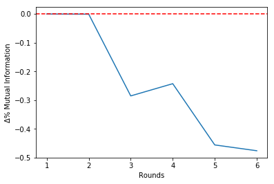
Making the selection choosing to stop at Round 2:
X_new = select.transform(X, rd=2)

X_new.shape
(10000, 5)
Categorizing :
ind0 = (y<np.percentile(y, 33))
ind1 = (np.percentile(y, 33)<=y) & (y<np.percentile(y, 66))
ind2 = (np.percentile(y, 66)<=y)

y[ind0] = 0
y[ind1] = 1
y[ind2] = 2

y=y.astype(int)y[:15]array([2, 0, 1, 2, 0, 2, 0, 0, 0, 1, 2, 1, 0, 0, 2])
Training (and validating) GMMs:
%%time

gmm=inf.get_gmm(X, y, y_cat=True)
Wall time: 6.7 s
Ordering features by their importances using the Forward Selection algorithm:
select=inf.SelectVars(gmm, selection_mode='forward')
select.fit(X, y, verbose=True)
Let's start...
Round = 0 | Î = 0.00 | Δ%Î = 0.00 | Features=[]
Round = 1 | Î = 0.14 | Δ%Î = 0.00 | Features=[3]
Round = 2 | Î = 0.28 | Δ%Î = 1.01 | Features=[3, 0]
Round = 3 | Î = 0.50 | Δ%Î = 0.79 | Features=[3, 0, 1]
Round = 4 | Î = 0.62 | Δ%Î = 0.22 | Features=[3, 0, 1, 4]
Round = 5 | Î = 0.75 | Δ%Î = 0.21 | Features=[3, 0, 1, 4, 2]
Round = 6 | Î = 0.75 | Δ%Î = -0.00 | Features=[3, 0, 1, 4, 2, 5]
Round = 7 | Î = 0.74 | Δ%Î = -0.01 | Features=[3, 0, 1, 4, 2, 5, 6]
Checking history:
select.get_info()| rounds | mi_mean | mi_error | delta | num_feat | features | |
|---|---|---|---|---|---|---|
| 0 | 0 | 0.000000 | 0.000000 | 0.000000 | 0 | [] |
| 1 | 1 | 0.139542 | 0.005217 | 0.000000 | 1 | [3] |
| 2 | 2 | 0.280835 | 0.006377 | 1.012542 | 2 | [3, 0] |
| 3 | 3 | 0.503872 | 0.006499 | 0.794196 | 3 | [3, 0, 1] |
| 4 | 4 | 0.617048 | 0.006322 | 0.224612 | 4 | [3, 0, 1, 4] |
| 5 | 5 | 0.745933 | 0.005135 | 0.208874 | 5 | [3, 0, 1, 4, 2] |
| 6 | 6 | 0.745549 | 0.005202 | -0.000515 | 6 | [3, 0, 1, 4, 2, 5] |
| 7 | 7 | 0.740968 | 0.005457 | -0.006144 | 7 | [3, 0, 1, 4, 2, 5, 6] |
It is possible to see that the estimated mutual information is untouched from Round 6 onwards.
Since there is a 'break' in Round 5, we should choose to stop the algorithm at theta round. This will be clear in the Mutual Information history plot that follows:
select.plot_mi()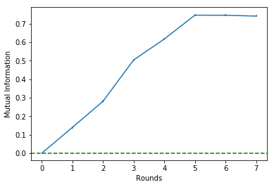
Plotting the percentual variations of the mutual information between rounds:
select.plot_delta()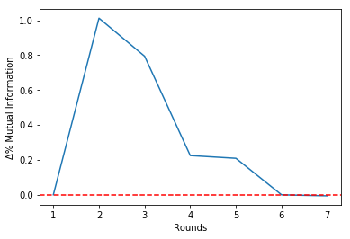
Making the selection choosing to stop at Round 5:
X_new = select.transform(X, rd=5)

X_new.shape
(10000, 5)
[1] Eirola, E., Lendasse, A., & Karhunen, J. (2014, July). Variable selection for regression problems using Gaussian mixture models to estimate mutual information. In 2014 International Joint Conference on Neural Networks (IJCNN) (pp. 1606-1613). IEEE.
[2] Lan, T., Erdogmus, D., Ozertem, U., & Huang, Y. (2006, July). Estimating mutual information using gaussian mixture model for feature ranking and selection. In The 2006 IEEE International Joint Conference on Neural Network Proceedings (pp. 5034-5039). IEEE.
[3] Maia Polo, F., & Vicente, R. (2022). Effective sample size, dimensionality, and generalization in covariate shift adaptation. Neural Computing and Applications, 1-13.