An Adaptive Simulated Annealing EM Algorithm for Inference on Non-homogeneous Hidden Markov Models
In this package we are adding adaptive simulated variable selection, and various prediction options for the standard depmixS4 (https://cran.r-project.org/web/packages/depmixS4/) for inference on non-homogeneous hidden Markov models (NHHMM). NHHMM are a subclass of dependent mixture models used for semi-supervised learning, where both transition probabilities between the latent states and the mean parameter of the probability distribution of the responses (for a given state) depend on the set of up to p covariates. A priori we do not know which (and how) covariates influence the transition probabilities and the mean parameters. This induces a complex combinatorial optimization problem for model selection with 4 to the power of p potential configurations. To address the problem, in this article we propose an adaptive (A) simulated annealing (SA) expectation maximization (EM) algorithm (ASA-EM) for joint optimization of models and their parameters with respect to a criterion of interest.
- Full text of the paper introducing An Adaptive Simulated Annealing EM Algorithm for Inference on Non-homogeneous Hidden Markov Models: ACM and arXiv
- Some applications of the package are available on: GitHub
- Install binary on Linux or Mac Os:
install.packages("https://github.com/aliaksah/depmixS4pp/blob/master/depmixS4pp_1.0.tar.gz?raw=true", repos = NULL, type="source")- An expert parallel call of parallel ASA-EM (see select_depmix):
results = depmixS4pp::select_depmix(epochs =3,estat = 3,data = X,MIC = stats::AIC,SIC =stats::BIC,family = gaussian(),fparam = fparam,fobserved = fobserved,isobsbinary = c(0,0,rep(1,length(fparam))),prior.inclusion = array(1,c(length(fparam),2)),ranges = 1,ns = ns,initpr = c(0,1,0),seeds = runif(M,1,1000),cores = M)- A simple call of prediction function (see predict_depmix):
y.pred = depmixS4pp::predict_depmix(X.test,object = results$results[[results$best.mic]]$model,mode = F)Consider an example of Apple (AAPL) stock price predictions
The example is focused upon Aple stock (AAPL) prediction with respect to log-returns of p=29 stocks from the S&P500 listing with the highest correlations to AAPL. The addressed data consists of 1258 observations of log returns for 30 stocks based on the daily close price. Th predictors are: "ADI", "AMAT", "AMP", "AOS", "APH", "AVGO", "BLK", "BRK.B", "CSCO", "FISV", "GLW", "GOOGL", "GOOG", "HON" "INTC", "ITW", "IVZ", "LRCX", "MA", "MCHP", "MSFT", "QRVO", "ROK", "SPGI", "SWKS", "TEL", "TSS", "TXN", "TXT", where the underscripts are representing the official S&P500 acronyms of the stocks. In terms of physical time, the observations are ranged from 11.02.2013 to 07.02.2018. The focus of this example is in both inference and predictions, hence we divided the data into a training data set (before 01.01.2017) and a testing data set (after 01.01.2017). The full data processing script is available at https://github.com/aliaksah/depmixS4pp/blob/master/examples/AAPL_example.R, but here let:
X #be the training data on 30 stocks
X.test #be the test data on 30 stocks
The primary model selection criterion addressed in this example is AIC due to that we are mainly interested in predictions, whilst BIC is the secondary reported criterion.
Then we specify initial formulas with all possible covariates for but the observed and latent processes as:
fparam = c("ADI", "AMAT", "AMP", "AOS", "APH", "AVGO", "BLK", "BRK.B", "CSCO", "FISV", "GLW", "GOOGL", "GOOG", "HON" "INTC", "ITW", "IVZ", "LRCX", "MA", "MCHP", "MSFT", "QRVO", "ROK", "SPGI", "SWKS", "TEL", "TSS", "TXN", "TXT")and the observations as
fobserved = "AAPL"We will run the ASA-EM with gaussian observations with 3 latent states on 30 cores. Specify:
ns = 3
M = 30
And run the inference with the stated in the call choice of tuning parameters of the algorithm:
results = depmixS4pp::select_depmix(epochs =3,estat = 3,data = X,MIC = stats::AIC,SIC =stats::BIC,family = gaussian(),fparam = fparam,fobserved = fobserved,isobsbinary = c(0,0,rep(1,length(fparam))),prior.inclusion = array(1,c(length(fparam),2)),ranges = 1,ns = ns,initpr = c(0,1,0),seeds = runif(M,1,1000),cores = M)Now we can make the predictions (conditional on the mode state of NHHMM) as:
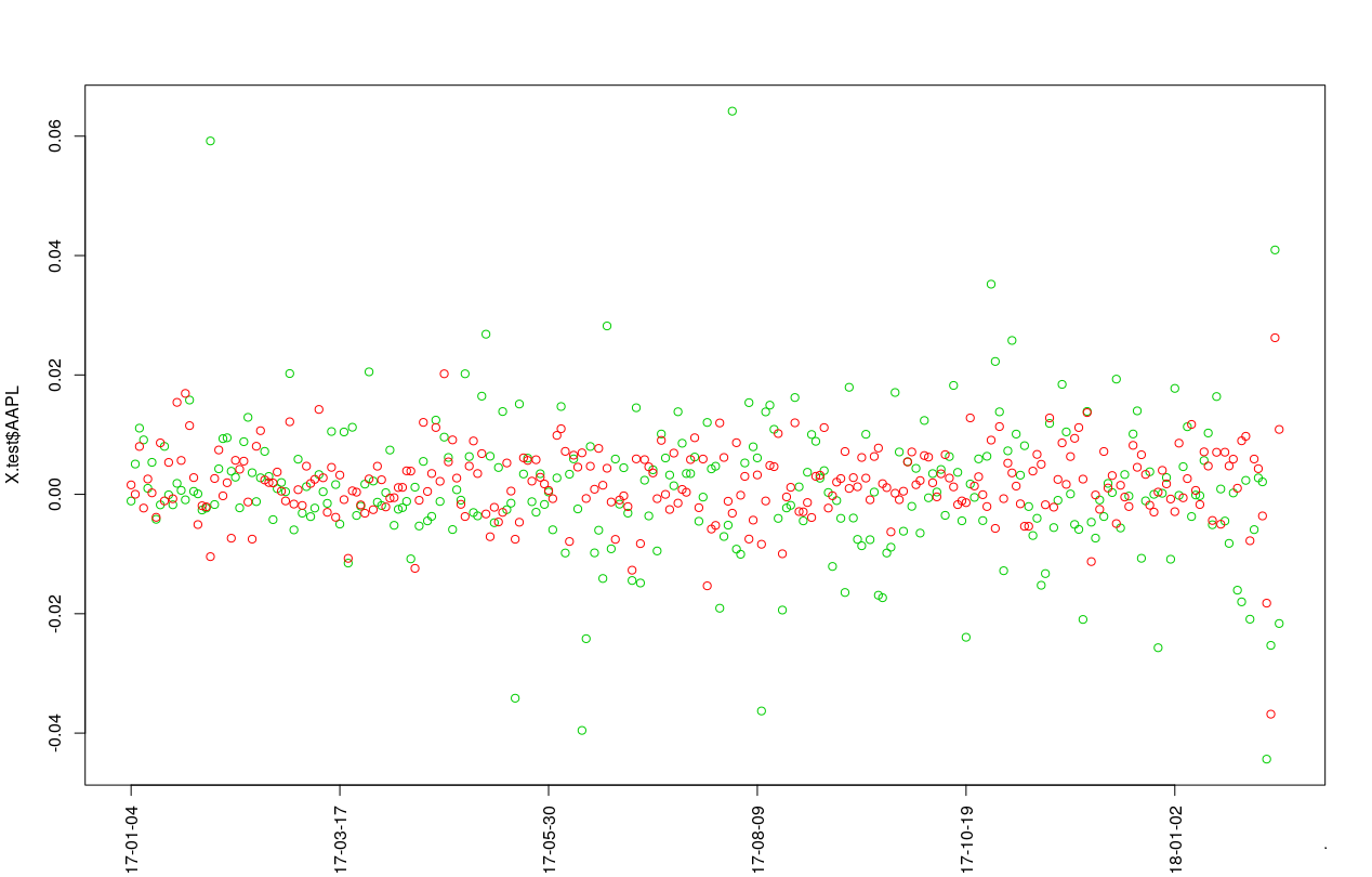
y.pred = depmixS4pp::predict_depmix(X.test,object = results$results[[results$best.mic]]$model,mode = T)And plot the predictions for the log-returns (red) and actual test log-returns (green):
plot(X.test$AAPL, col =3,xaxt = "n")
points(y.pred$y, col = 2)
axis(1, at=seq(1,length(X.test$AAPL), by = 50), labels=X.test$date[seq(1,length(X.test$date), by = 50)],las=2)
prc = sp*exp(cumsum(X.test$AAPL))
prc.pred = sp*exp(cumsum(y.pred$y))
And plot the predictions for the price (blue) and actual test price (brown) via:
plot(prc,col = "brown",type = "l",ylim = c(100,200),xaxt = "n")
lines(prc.pred, col = "blue")
axis(1, at=seq(1,length(X.test$AAPL), by = 50), labels=X.test$date[seq(1,length(X.test$date), by = 50)],las=2)
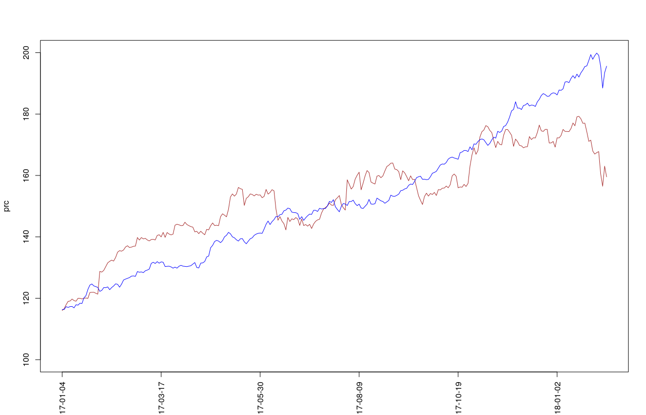
mse.hmm.pr = sqrt(mean((prc.pred-prc)^2))Benchmarks against other methods can be found here.
Additionally the research was presented via the following selected contributions:
Scientific lectures
-
Hubin, Aliaksandr; Storvik, Geir Olve. On model selection in hidden Markov models with covariates. Workshop, Klækken Workshop 2015; Klækken, 29.05.2015.
-
Hubin, Aliaksandr; An adaptive simulated annealing EM algorithm for inference on non-homogeneous hidden Markov models. International Conference on Artificial Intelligence (AIIPCC 2019), Information Processing and Cloud Computing; Sanya, 20.12.2019.
Bibtex Citation Format:
inproceedings{Hubin:2019:ASA:3371425.3371641,
 author = {Hubin, Aliaksandr},
 title = {An Adaptive Simulated Annealing EM Algorithm for Inference on Non-homogeneous Hidden Markov Models},
 booktitle = {Proceedings of the International Conference on Artificial Intelligence, Information Processing and Cloud Computing},
 series = {AIIPCC '19},
 year = {2019},
 isbn = {978-1-4503-7633-4},
 location = {Sanya, China},
 pages = {63:1--63:9},
 articleno = {63},
 numpages = {9},
 url = {http://doi.acm.org/10.1145/3371425.3371641},
 doi = {10.1145/3371425.3371641},
 acmid = {3371641},
 publisher = {ACM},
 address = {New York, NY, USA},
 keywords = {adaptive parameter tuning, expectation maximization, hidden Markov models, model selection, simulated annealing},
}