fabge / stock_market_prediction

An exercise in trying to predict the stock market with neural nets.

Predicting the stock market

This blogpost aims to give a short overview of trying to predict the stock market with neural networks. At first the desired data has to be aquired. Fortunately the pandas_datareader library makes it easy to access the Yahoo API and make a request. The aquired data consists of the S&P500, which is an American stock market index based on the market capitalizations of 500 large companies having common stock listed on the NYSE or NASDAQ (wiki) and the Apple stock market data. The timespan ranges from the 1st January 1995 until the 30th September 2018.

Inspiration and reference from here and there.

Import the data

import numpy as np
import pandas as pd
import matplotlib.pyplot as plt

import pandas_datareader as pdr

%matplotlib inline

sp500_data = pdr.get_data_yahoo("^GSPC", "1995-01-01", "2018-09-30")
apple_data = pdr.get_data_yahoo("AAPL", "1995-01-01", "2018-09-30")

As we can see, we have 5979 datapoints and 6 Attributes in total.

sp500_data.info()

<class 'pandas.core.frame.DataFrame'>
DatetimeIndex: 5979 entries, 1995-01-03 to 2018-09-28
Data columns (total 6 columns):
High         5979 non-null float64
Low          5979 non-null float64
Open         5979 non-null float64
Close        5979 non-null float64
Volume       5979 non-null int64
Adj Close    5979 non-null float64
dtypes: float64(5), int64(1)
memory usage: 327.0 KB

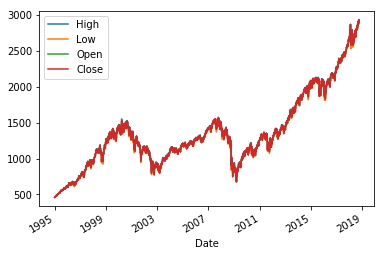
The plot below shows the performance of the S&P500 over the last 13 years. Global crises (around 2008) or other recessions can be recognized easily.

sp500_data[['High', 'Low', 'Open', 'Close']].plot()

<matplotlib.axes._subplots.AxesSubplot at 0x1075cb898>

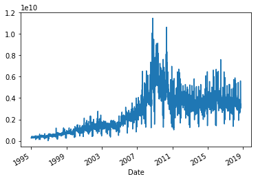
The volume attribute gives us "the amount (total number) of a security (or a given set of securities, or an entire market) that was traded during a given period of time." (wiki)

sp500_data['Volume'].plot()

<matplotlib.axes._subplots.AxesSubplot at 0x108d45048>

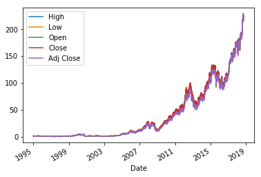
apple_data.drop('Volume', axis=1).plot()

<matplotlib.axes._subplots.AxesSubplot at 0x10e67f630>

apple_data.head()

<style scoped> .dataframe tbody tr th:only-of-type { vertical-align: middle; }

.dataframe tbody tr th {
    vertical-align: top;
}

.dataframe thead th {
    text-align: right;
}

</style>

	High	Low	Open	Close	Volume	Adj Close
Date
1995-01-03	1.388393	1.352679	1.388393	1.370536	25967200.0	1.200917
1995-01-04	1.415179	1.379464	1.379464	1.406250	39670400.0	1.232210
1995-01-05	1.406250	1.383929	1.401786	1.388393	18410000.0	1.216563
1995-01-06	1.540179	1.468750	1.486607	1.500000	269155600.0	1.314358
1995-01-09	1.495536	1.464286	1.486607	1.471539	68521600.0	1.289419

Prepare training, validation and test data

When the dataset consists of data with a time-reference, creating training and test sets from randomly sampling the data is not a good idea most of the time. Rachel Thomas talks about the specifics in detail in her blogpost.

The following code snippet splits the data into 80% train, 10% test and 10% validation data.

def train_test_val_split(data):
    #data = data[['High', 'Low', 'Open', 'Close']]
    data = data['Close']
    n_test_samples = int(len(data)*0.1)
    n_val_samples = int(len(data)*0.1)
    
    train = data[:-(n_val_samples+n_test_samples)]
    val = data[-(n_val_samples+n_test_samples):-n_test_samples]
    test = data[-n_test_samples:]
    return train, val, test

train, val, test = train_test_val_split(apple_data)

train = train[:,None]
val = val[:,None]
test = test[:,None]

train.shape, val.shape, test.shape

((4785, 1), (597, 1), (597, 1))

Scale the data

Neural networks "behave nicely" when the input data is scaled. It is important to apply the same scaling to train and test.

from sklearn.preprocessing import MinMaxScaler
scaler = MinMaxScaler()
scaler.fit(train)
train = scaler.transform(train)
val = scaler.transform(val)
test = scaler.transform(test)

train.shape, val.shape, test.shape

((4785, 1), (597, 1), (597, 1))

train = np.squeeze(train)
val = np.squeeze(val)
test = np.squeeze(test)

Generate dependent and independet variables regarding sequence length

Because we focus on the Closing Price of the stock or index, we only have one attribute for training and test purposes. This means, we have to create our own dependent and independet variables. The follow code snippet takes the seq_len attribute and creates the variables as follows:

• 10 consecutive days are put into an array, this will be the first row of X_train
• the day after the last day in X_train, so the 11th day is put into y_train

The creation of the variables as described above means, we want to train an algorithm by giving 10 days of stock market data and want it to predict the 11th day.

def gen_data(data, seq_len):
        """
        Generates training data
        :param seq_len: length of window
        :return: X_train and Y_train
        """
        X_train, y_train = [], []
        for i in range((len(data)//seq_len)*seq_len - seq_len - 1):
            x = np.array(data[i: i + seq_len])
            y = np.array([data[i + seq_len + 1]], np.float64)
            X_train.append(x)
            y_train.append(y)
        return np.array(X_train), np.array(y_train)

X_train, y_train = gen_data(train, 10)
X_val, y_val = gen_data(val, 10)
X_test, y_test = gen_data(test, 10)

X_train.shape

(4769, 10, 1)

Construct neural network with Keras (MLP)

We define a neural network with Tensorflow and Keras. Keras makes it very easy to put together a neural network in a very modular way. The architecture in the code snippet below is called a multilayer perceptron and consists of the most basic components of a neural net.

import tensorflow as tf

model = tf.keras.models.Sequential()
model.add(tf.keras.layers.Dense(50, input_dim=10, activation=tf.nn.relu))
model.add(tf.keras.layers.Dense(50, activation=tf.nn.relu))
model.add(tf.keras.layers.Dense(1, activation=tf.nn.relu))

model.compile(optimizer="adam", loss="mean_squared_error")

model.fit(X_train, y_train, validation_data=(X_val, y_val), epochs=100, verbose=0)

<tensorflow.python.keras.callbacks.History at 0x1c4be6c470>

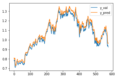
y_val_pred = model.predict(X_val)

plt.plot(y_val)
plt.plot(y_val_pred)
plt.legend(['y_val', 'y_pred'], loc='best')

<matplotlib.legend.Legend at 0x1c4bfad588>

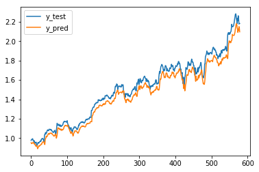
y_test_pred = model.predict(X_test)

As one can see, the neural net fits the curve of the test set quite well, yet it must be said that predicting only a single day makes the curve fit pretty closely anyways.

plt.plot(y_test)
plt.plot(y_test_pred)
plt.legend(['y_test', 'y_pred'], loc='best')

<matplotlib.legend.Legend at 0x1c4c0b3128>

I will dive into this deeper in the future.
Following points need to be adressed:

• read more into how to properly construct dependet and independet variable in stock prediction scenarios
• change the timespans of X and y
• consider other architectures, such as LSTM or other, deeper neural networks