esaucedof / colorfindr

Extracts colors from various image types, plots treemaps and 3D scatterplots of color compositions, create color palettes.

colorfindr

This R package allows you to extract colors from various image types (currently JPEG, PNG, TIFF, SVG, BMP). Either a tailored report (directly with the main function get_colors), a treemap (plot_colors) or a 3D scatterplot (plot_colors_3d) with the image color composition can be returned. Version 0.1.4 provides several methods for creating discrete color palettes.

Installation

Version 0.1.4 is on CRAN and can be installed as follows:

install.packages("colorfindr")

Install from GitHub for a regularly updated version (latest: 0.1.4):

install.packages("devtools")
devtools::install_github("zumbov2/colorfindr")

Treemap examples

Color composition of the South African flag

Code

# Load packages
pacman::p_load(colorfindr, dplyr)

# Plot
get_colors(
  img = "https://upload.wikimedia.org/wikipedia/commons/a/af/Flag_of_South_Africa.svg",
  min_share = 0.05
) %>%
  plot_colors(sort = "size")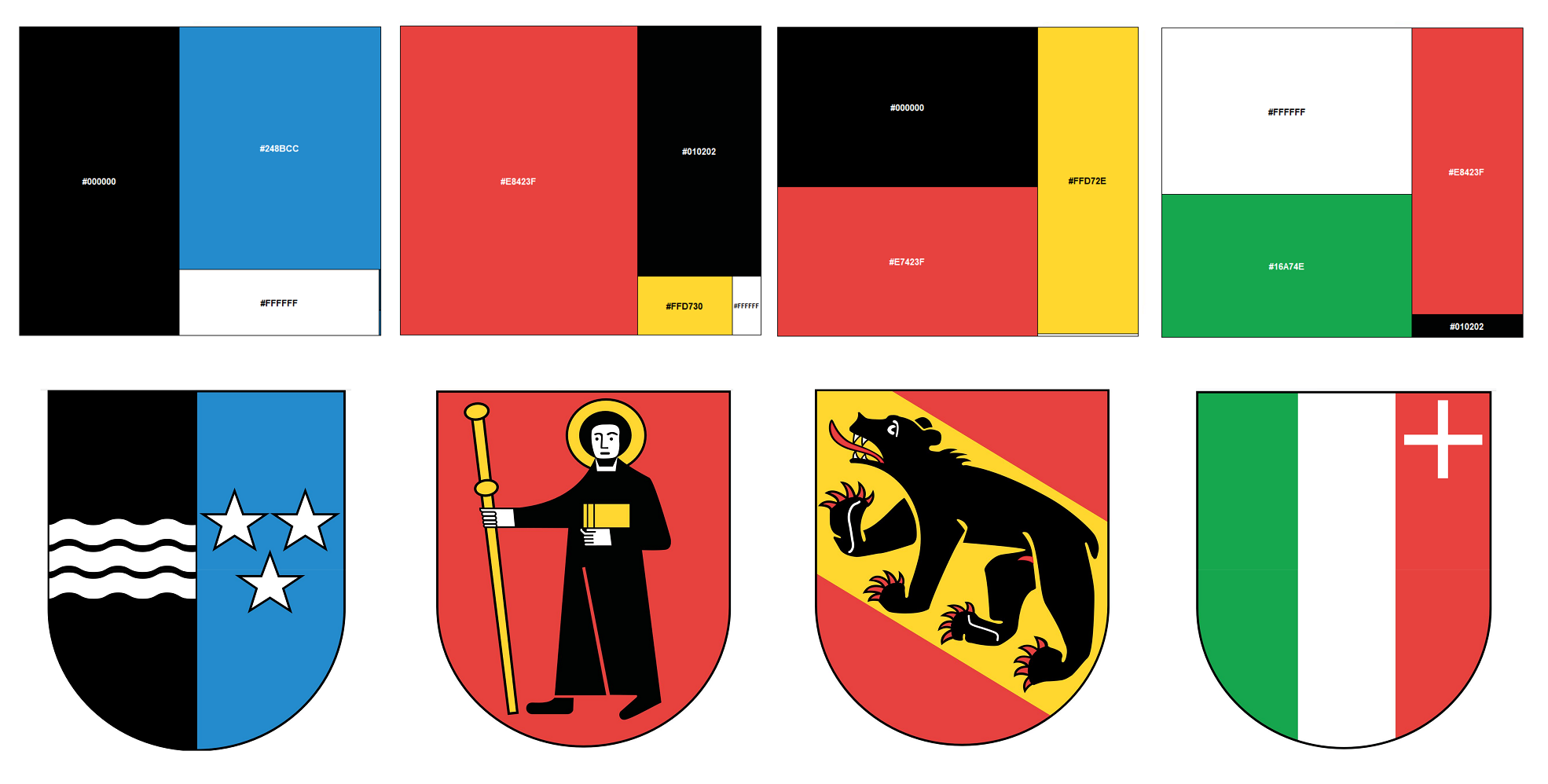

Flags of Swiss Cantons

Code

# Load packages
pacman::p_load(colorfindr, dplyr)

# Images
img <- c(
  "https://upload.wikimedia.org/wikipedia/commons/b/b5/Wappen_Aargau_matt.svg",
  "https://upload.wikimedia.org/wikipedia/commons/0/0e/Wappen_Glarus_matt.svg",
  "https://upload.wikimedia.org/wikipedia/commons/4/47/Wappen_Bern_matt.svg",
  "https://upload.wikimedia.org/wikipedia/commons/d/d1/Wappen_Neuenburg_matt.svg"
)

# Plot
for (i in 1:length(img)) get_colors(img[i], top_n = 4) %>% plot_colors(sort = "size")

3D Scatterplot examples

This part of the package was inspired by the wonderful plots of alfieish. They caused a sensation on Reddit in autumn 2017. The plots are created with Plotly and are accordingly interactive.

Color composition of Edvard Munch's The Scream

The original can be found under: https://plot.ly/~zumbov/14.embed.

Code

# Load packages
pacman::p_load(colorfindr, dplyr)

# Plot (5000 randomly selected pixels)
get_colors("https://upload.wikimedia.org/wikipedia/commons/f/f4/The_Scream.jpg") %>% 
  plot_colors_3d(sample_size = 5000, marker_size = 2.5, color_space = "RGB")

Color composition of Salvador Dalí's The Persistence of Memory

The original can be found under: https://plot.ly/~zumbov/20.embed.

Code

# Load packages
pacman::p_load(colorfindr, dplyr)

# Plot (5000 randomly selected pixels)
get_colors("http://wisetoast.com/wp-content/uploads/2015/10/The-Persistence-of-Memory-salvador-deli-painting.jpg") %>%
  plot_colors_3d(sample_size = 5000, marker_size = 2.5, color_space = "RGB")

Read more here on how to publish your graphs to Plotly.

Other masterpieces

Da Vinci's Mona Lisa -> Color composition
Vermeer's Girl with a Pearl Earring -> Color composition
Klimt's The Kiss -> Color composition
Van Gogh's The Starry Night -> Color composition

Different color spaces

From version 0.1.2 on it is possible to display the point clouds in different color spaces: Besides ...

RGB

HSV (hue, saturation, value) and ...

HSL (hue, saturation, lightness) ...

are available.

Code

# Load packages
pacman::p_load(dplyr, colorfindr)

# Get colors
col <- get_colors("http://joco.name/wp-content/uploads/2014/03/rgb_256_1.png")

# Plot to alternative color spaces
plot_colors_3d(col, color_space = "RGB")
plot_colors_3d(col, color_space = "HSV")
plot_colors_3d(col, color_space = "HSL")

Creating color palettes

Version 0.1.4 provides various methods for creating color palettes with a distinct number of colors. The default method performs a k-means clustering on the pixels in the RGB color space (clust_method = "kmeans"). Alternatively, the pixel clusters can be created with a version of the median cut algorithm (clust_method = "median_cut"). The user can also choose whether the most common RGB combination per cluster is extracted (default: extract_method = "hex_freq") or whether new RGB combinations are created for each cluster, either based on the mean (extract_method = "mean"), median (extract_method = "median") or mode (extract_method = "mode") of the RGB dimensions. The default has the advantage that the extracted colors actually appear in the image used. For images with many color nuances, however, the other extraction methods seem to achieve more convincing results.

Childhood memories I

Code

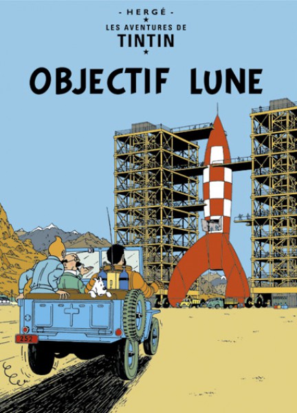
# Load packages
pacman::p_load(dplyr, colorfindr)

# Ensure reproducibility
set.seed(123)

# Get colors and create a palette with n = 5 
get_colors("https://www.movieart.ch/bilder_xl/tintin-et-milou-poster-11438_0_xl.jpg") %>% 
make_palette(n = 5)

Childhood memories II

Code

# Load packages
pacman::p_load(dplyr, colorfindr)

# Ensure reproducibility
set.seed(123)

# Get colors and create a palette with n = 5 
get_colors("http://www.coverbrowser.com/image/lucky-luke/5-1.jpg") %>% 
    make_palette(n = 5)

Vintage ads from Switzerland I

Code

# Load packages
pacman::p_load(dplyr, colorfindr)

# Ensure reproducibility
set.seed(123)

# Get colors and create a palette with n = 5 
get_colors("http://www.gallery29.ie/images/posters/1171469398_DSC03889.jpg") %>% 
    make_palette(n = 5)

Vintage ads from Switzerland II

Code

# Load packages
pacman::p_load(dplyr, colorfindr)

# Ensure reproducibility
set.seed(123)

# Get colors and create a palette with n = 5 
get_colors("https://www.artifiche.com/cms/upload/posters_extralarge/2850.jpg") %>% 
    make_palette(n = 5)

Happy Testing!