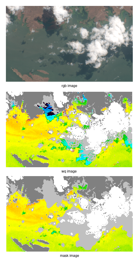
Satellite images can be used to calculate water quality and depth. Most steps in this process are fully automated, but it is still essential that in the last step, a geographer reviews the calculated results and flags out certain parts of the image, if necessary. Causes for this are cloud shadows, which make pixels darker than they actually are, sun glint, and some others. Our project aims to automate the final reviewing process by training a convolutional neural network ( e.g. U-Net) to predict the correct label for each pixel (Semantic Image Segmentation).
todo: add graphic
To get started with this project, follow the steps below: We are using poetry as a dependency manager.
Requirements: Python 3.10 ≤
Install poetry
-
Clone the repository using
git clone <repository_url>. -
Activate poetry virtual environment.
# Create a virtual environment
$ poetry shell
# Install all packages
$ poetry install
Our dataset contains large satellite images taken from the reservoir Lake Cahora Bassa in Mozambique at 15 different times. The satellite images are RGB images with an additional alpha channel. In addition to the satellite images, the dataset includes a water-quality image (wq image) with one channel and a mask image with one channel for each timestamp.
The water quality image and the mask image contain one channel valued between 0 and 255.
- All pixels with 253 and 255 are labeled as invalid.
- All pixels with value 0 are labeled as land.
- The rest of the pixels are labeled as valid.
As the example images show that the wq image is already partly flagged. The white parts represent the clouds while the gray parts represent cloud shadows. However the flagging is not the same as in the mask image. A geologist manually adapts the flagging with his expertise. The challenge of this project is to train a neural network so that the result is closer to the mask image than the wq image.
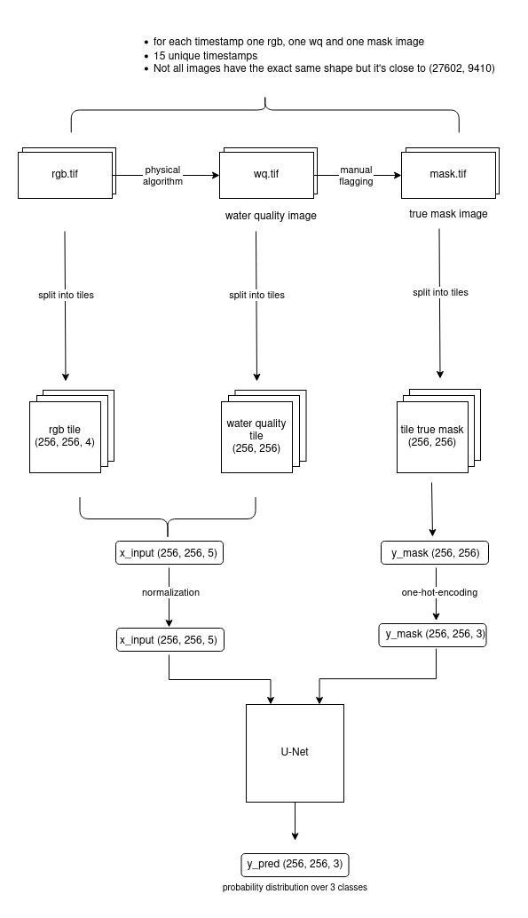
To train our machine learning model we combined the rgb images and the water quality images into one input image with 5 channels. As the size of each image is too large to use it as input for the neural network we split each image into smaller tiles of size 256 x 256 once with an overlap of 56 pixels and once without overlapping.
Our dataset is imbalanced, meaning the number of pixels per label differ:
- Mean percentage of invalid tiles: 23.48 %
- Mean percentage of valid tiles: 31.89 %
- Mean percentage of land tiles: 44.63 %
For more details check out the data exploration notebook
As we did not have any inconsistencies or missing values in our dataset we only had to
- remove irrelevant data (tiles that only contained land pixels were removed)
- create mask (pixel values needed to be translated into labels)
- normalize data (rgb channels needed to be normalized as unet works best with input values between 0 and 1)
- one-hot-encoding
To split the images into tiles, follow these steps:
- Create an empty
/datafolder in the project root directory. - Copy the two subfolders
unflaggedandflags_appliedfrom the original data folder into the project/datafolder. - Create a
.envfile in the root directory and define theDATA_PATHvariable - Run
main.pyin the/prepare_datadirectory to prepare the data for analysis.
The result is a folder named /google_drive that contains one compressed file per date. Each file consists of the true_mask array and the x_input array which are used to train the neural network.
- Execute the
/full_dataset_splitting_mmaps.ipynbnotebook
In this folder, all models used for training are saved and some additional helper function. To train our network used the u-net architecture.
All experiments that have been done are saved here.
In this folder we explored our dataset to know about the class imbalance, number of tiles per image and the overlap between the input image and the true mask (physics_jaccard).
This folder contains all helper methods and functions to calculate metrics for each trained folder which are saved on google drive.
The model performance is evaluated with the Intersection over Union (Jaccard Index) because the dataset is imbalanced which means that accuracy might be biased towards the larger class, whereas the Jaccard Index provides a more accurate measurement of similarity between predicted and actual labels. The Intersection over Union is calculated for each label separately. To evaluate the model performance the mean for all 3 labels is calculated. In addition to the Jaccard Index the F1 Score, Precision, Recall and specificity are also calculated and used to evaluate the model performance. to get an insight into the true positive rate, the ratio between true positives and false negatives and the true negative rate.
As the unet architecture is very popular for semantic segmentation problem I started with a u-net architecture very similar to the original architecture except that I used one convolutional layer less to make the training faster in the beginning.
Experiment 1 explores the variance when training multiple models with the same configuration. To simplify the setup and get familiar with the libraries only a small subset of the entire dataset with overlapping tiles was used. Experiment 2 is similar to experiment 1 except for the dataset, as non-overlapping tiles were used instead.
In experiment 3 the entire dataset was used for the training. As the RAM capacity was not sufficient DataGenerators were used so that the data was loaded in batches into RAM. Three models were trained with slightly different training configurations. The training of model 0 was stopped to early which led to underfitting while the training of model 1 was too long which led to overfitting. Model 2 was trained with an adjusted early stopping rate (10 instead of 5 as in model 1), adjusted callback that monitors validation accuracy and loss and a checkpoint callback which saves the model after the best performing epoch. The best performing model can make predictions with a mean intersection over union of `0.935624. The aim of experiments 4 and 5 was to explore variance in the training. Therefore, 5 models each for overlapping and non-overlapping tiles were trained with the optimized configuration of experiment 3. As the variance was lower and the mean intersection over union was slightly better for the non-overlapping dataset all further experiments continue with the non-overlapping dataset.
The goal of the following experiments is to get familiar with hyperparameters, to find the optimal combination of hyperparameters. I split the hyperparameters into three different categories:
Training Configuration
- Number of Epochs (experiment_3)
- Callbacks (experiment_3)
- Optimizer (experiment 7)
- Learning rate (experiment 7)
- Batch size
Model Parameters
- amount of conv2d layers (experiment 8)
- activation functions
Overfitting avoidance
- dropout (experiment 9)
My approach was to find a good training configuration first and then move on to optimize the unet architecture
before experimenting with regularization methods.
In experiment 6 the early
stopping callback was optimized to check the mean intersection over union and the loss
instead of the accuracy.
In experiment 7 different
optimizers with different learning rates were tested. Given the resources AdamW performed
best. The best model could perform with a jaccard index of 0.951696. At this point a good training configuration was
found and I moved on to optimizing the unet architecture.
In experiment 8 I tested
different amounts of Conv2D layers with different amounts of filter sizes. Only the
architecture with one convolutional layer less than the original performed better than the one I started with. The
intersection over union could be improved to `0.95598.
The first unet trained on the entire dataset performed with an intersection over union of 0.927125. After
hyperparameter
optimization the metric could be improved to 0.951696
As a benchmark, the overlap between the wq image and the final mask image was calculated. The mean intersection over
union for the test data is 0.897474.
Only edit and push jupyter notebooks on google colab, edit and push .py scripts always locally!
As it is only possible to push changes on jupyter notebooks to github from google colab it is best to do all changes in the scripts locally. Run all the prepare data scripts locally and only store the final numpy array in google drive.
- The MachineLearning folder will appear in your google drive
shared with mesubfolder. To access it from within colab you need to create a shortcut. (left click on the folder, 'add shortcut')

