Data Science in Python Tutorial

Karl-Ludwig Poggemann - labyrinthine circuit board lines –** Photo - CC BY 2.0
Data science is a sizzling hot field. According to the Harvard Business Review in 2012, it’s The Sexiest Job of the 21st Century. Even though there’s no standard definition of what data science is, most definitions typically refer to it as an interdisciplinary field that encompass computer science, statistics, machine learning, research, and analytics. In order for someone to become an effective data scientist, they must be able to extract knowledge or insights from data in various forms. In this section you’ll get an intro to Pandas, NumPy, and Matplotlib.
Pandas
Pandas can be described as an open source Python library for data manipulation and analysis. The name panda is not inspired by the fluffy bear who feasts on bamboo, but instead "panel data" which is an econometrics term. Installing Pandas with a prepackaged solution like Anaconda is probably the most straightforward option. Below are more options on how to install panda:
Installation from PyPI
The pandas library can be installed by PyPI using the following command:
pip install pandas
Installation on Linux
If you’re working on a Linux distro and refuse to use any prepackaged solution then you can install from the terminal:
Debian and Ubuntu:
sudo apt-get install python-pandas
Fedora:
zypper in python-pandas
To check that pandas installed correctly type in the following statement:
import pandas
If no error occurs then pandas have been successfully installed.
Panda Data Structures: Series and DataFrames
At the focal point of pandas are two data structures which are Series and DataFrame. A Series can be described as an arrangement of one-dimensional data containing a sequence of values, and a DataFrame which is the main object of panda is a two-dimensional tabular data structure.
Here’s an example of a Series:
>>> import pandas as pd
>>> s = pd.Series([1,5,10,15,20])
>>> s
0 1
1 5
2 10
3 15
4 20
dtype: int64
The pandas library is imported as pd. Then, a Series is created, which is a one-dimensional labeled array that can hold a mixture of data types such as integer, floating points, strings, tuples, etc. As you can see, Series are indexed like lists or tuples. You can access the values by using the subscript notation as shown below:
>>> s[1]
5
>>> s[3]
15
>>> s[-1]
ERROR!
A series has a host of attributes and methods that you can use to access data and manipulate it as shown in the following code fragment:
>>> s.size
5
>>> s.values
array([ 1,  5, 10, 15, 20])
>>> s.ndim
1
>>> s.imag
array([0, 0, 0, 0, 0])
>>> s.is_unique
True
>>> s.tail(2)
3    15
4    20
>>> s.to_csv('/home/usr/Desktop/Series.csv')
Download Series.csv on GitHub.
DataFrame
The primary pandas data structure is known as the DataFrame. A DataFrame is as a rectangular table of two-dimensional, mutable, potentially heterogeneous data. It has labeled axes aka rows/columns, and according to the pandas docs, it can be thought of as a dict-like container for Series objects.
Let’s use numpy which you’ll learn more about in the next section to create one.
>>> import pandas
>>> data = pandas.DataFrame([0,1,2,3])
>>> data
0
0 0
1 1
2 2
3 3
The above creates a 4 x 4 DataFrame that randomly selects numbers in the range of 0-100.
The following snippet creates a DataFrame that compares the temperatures of Los Angeles and San Francisco from 2012-2017:
>>> import pandas as pd
>>> dates = pd.date_range('04-03-2012','04-08-2012')
>>> cities = pd.DataFrame({'Los Angeles':[75,72,64,72,82,79], 'San Francisco':[63,57,54,57,64,63]}, dates)
>>> cities
          Los Angeles  San Francisco
2012-04-03           75             63
2012-04-04           72             57
2012-04-05           64             54
2012-04-06           72             57
2012-04-07           82             64
2012-04-08           79             63
In the above program the pandas library is imported as pd. The date_range() function is used in order to create a range of dates to analyze. Then, a DataFrame is created from two dictionaries, one to represent the city of Los Angeles during those time periods, and another to represent the city of San Fran. We can use various operators and functions to manipulate the data and generate insights from it. For example, to get the difference in temperature for each day do the following:
>>> cities['Los Angeles'] - cities['San Francisco']2012-04-03 12
2012-04-04 15
2012-04-05 10
2012-04-06 15
2012-04-07 18
2012-04-08 16
Freq: D, dtype: int64
To return the cities back in a specific order do the following:
>>> cities[['San Francisco', 'Los Angeles']] San Francisco Los Angeles
2012-04-03 63 75
2012-04-04 57 72
2012-04-05 54 64
2012-04-06 57 72
2012-04-07 64 82
2012-04-08 63 79
And, if you want to access just the temperatures of Los Angeles do the following:
>>> cities['Los Angeles']2012-04-03 75
2012-04-04 72
2012-04-05 64
2012-04-06 72
2012-04-07 82
2012-04-08 79
Freq: D, Name: Los Angeles, dtype: int64
If you want to find the average use the mean() function of pandas.DataFrame.
>>> cities.mean()Los Angeles 74.000000
San Francisco 59.666667
dtype: float64
NumPy
NumPy is a library for Python that includes support for computing large multidimensional arrays and matrices. NumPy is now considered the library of choice for scientific computing, and has a suite of functions for performing high-level calculations on arrays in an efficient manner. At the time of publication NumPy is open sourced under the BSD license. It has a large and active community making it a smart investment in your technical career.
NumPy Installation
If you have Python installed then you may already have NumPy as it’s often included in many Python distributions. To test that it’s installed open up a terminal, type python3, and then enter the following command:
>>> import numpy as npIf nothing happens then that’s great as NumPy is installed, if not then bummers, you have some work to do. There are plethoras of ways in which you can install NumPy:
- Windows: I’ll recommend using Conda as a quick and easy way to get NumPy installed on your machine:
- conda install numpy
- Linux: You can install NumPy through the terminal:
- Linux(Ubuntu and Debian): sudo apt-get install python-numpy
- Fedora: sudo yum install numpy scipy
- OS X: Go to the terminal and type:
- pip3 install numpy
Once NumPy is installed, test that everything works properly by opening up the terminal and typing the following:
>>> import numpy as npIf no errors occur then NumPy is officially installed.
The focal point of NumPy – The ndarray
There are many paths we can take to create a ndarray, so let’s start with the easiest one. A simple way to create an ndarray is to call the array() function and then pass a list into it as shown below:
>>> import numpy as np
>>> arr = np.array([1,2,3])
>>> arr
array([1, 2, 3])
As you can see from the code snippet the numpy library was imported as np, and then the array() function was called on np and then saved in a variable named arr. Let’s explore some of the built in attributes and functions of the ndarrays:
>>> arr.size
3
>>> arr.shape
(3,)
>>> arr.dtype
dtype('int64')
>>> arr.ndim
1
Below are more functions that can be applied to a ndarray:
>>> arr.reshape(3,1)array([[1],
[2],
[3]])
>>> arr.sum()6
>>> arr.fill(100)
>>> arr
array([100, 100, 100])
>>> arr.put(0,250)
>>> arr
array([250, 100, 100])
The reshape() function changes the shape of the ndarray so in this case it’s given three rows and one column, the sum() function adds up all of the elements of the array, the fill() function fills the elements with a certain value, and the put() function places a value at a certain position in the array.
The following shows how to create a 2D ndarray:
>>> arr = np.array([[1,2,3],[4,5,6]])
>>> arr
array([[1, 2, 3],
[4, 5, 6]])
>>> arr.ndim2
As you can see the number of square brackets you pad onto the array represents the number of dimensions it has. Therefore, what do you think will be the dimension of the following ndarray?
>>> arr = np.array([[[1,2,3],[4,5,6],[7,8,9]]])The answer is three. What about the shape? The answer is…
>>> arr.shape(1, 3, 3)
Slicing
Like lists, you can slice an ndarray by using the colon [:] syntax, but unlike lists the arrays created by slicing are not copies. Let’s look at the following array as an example:
>>> a = np.arange(1,11)The output is:
>>> aarray([ 1, 2, 3, 4, 5, 6, 7, 8, 9, 10])
The first element corresponds to index 0, and the last element corresponds to the size of the list which in this case is 10. Therefore, if you want to slice the elements from 6 through 10, one solution is to use the following:
>>> a[5:10]array([ 6, 7, 8, 9, 10])
Also, you can specify the step in each sequence with a third parameter as shown in the following examples:
>>> a[1::2]array([ 2, 4, 6, 8, 10])
>>> a[0::2]array([1, 3, 5, 7, 9])
In a[1::2] the array is sliced at its index 1 which is 2, and then it increments by 2 every subsequent step until it reaches the end of the list or at 10. In a[0::2], the list starts at 1, and increments by 2 all the way up to the end of the list which in this case is 9.
Let’s take a look at the following example:
>>> i = np.arange(1,41).reshape(10,4)
>>> i
array([[ 1, 2, 3, 4],
[ 5, 6, 7, 8],
[ 9, 10, 11, 12],
[13, 14, 15, 16],
[17, 18, 19, 20],
[21, 22, 23, 24],
[25, 26, 27, 28],
[29, 30, 31, 32],
[33, 34, 35, 36],
[37, 38, 39, 40]])
In the above example we have an ndarray with ten rows and four columns. What would the syntax be if we wanted to slice just the first row? The answer would look like the following:
>>> i[:1]array([[1, 2, 3, 4]])
Therefore, with this in mind if you wanted to slice through every other row in the matrix you would use the following syntax:
>>> i[::2]array([[ 1, 2, 3, 4],
[ 9, 10, 11, 12],
[17, 18, 19, 20],
[25, 26, 27, 28],
[33, 34, 35, 36]])
Ok, things are making sense, but how do one go about slicing columns? Well, columns like rows have indexes, and they also start at 0. Therefore, to access all of the elements of the first column of i, the syntax would be as follows:
>>> i[:,0]array([ 1, 5, 9, 13, 17, 21, 25, 29, 33, 37])
If you wanted to access just the first five elements of the first column, the syntax would instead be:
>>> i[0:5,0]array([ 1, 5, 9, 13, 17])
Iterating over ndarrays
Let's assume that we have an ndarray defined as follows:
>>> x = np.arange(1,11).reshape(5,2)
>>> x
array([[ 1, 2],
[ 3, 4],
[ 5, 6],
[ 7, 8],
[ 9, 10]])
When you use a normal for loop you can traverse all of the rows of a ndarray as shown below:
for elements in x:
    print(elements)
[1 2]
[3 4]
[5 6]
[7 8]
[9 10]
If you need to access the elements of the first column you can use a for loop as follow:
for elements in x:
    print(elements[0])
1
3
5
7
9
To get the elements of the second column use the following syntax:
for elements in x:
    print(elements[1])
2
4
6
8
10
You could also use the flat property to iterate over the array step-by-step.
for item in x.flat:
    print(item)
1
2
3
4
5
6
7
8
9
10
Below is a simple example that shows how to sum the elements of each column:
col_1 = 0
col_2 = 0
for elements in x:
    col_1 += elements[0]
    col_2 += elements[1]
>>> print("summation of col_1 =", col_1)
summation of col_1 = 25
>>> print("summation of col_2 =", col_2)
summation of col_2 = 30
NumPy provides an alternative to the for loop which is the apply_along_axis() function. This accepts three parameters and the first three arguments of the function are the aggregate function, the axis, and the array – if the axis is equal to 0 (default) the function is applied on the columns, and if it’s equal to one then it’s applied on the rows as shown below:
>>> np.apply_along_axis(lambda x: (x*3)/2,axis=1,arr=x)array([[ 1.5, 3. ],
[ 4.5, 6. ],
[ 7.5, 9. ],
[10.5, 12. ],
[13.5, 15. ]])
Input and output with NumPy
NumPy provides several functions that allow you to save the results in a binary text file, and it enables the reading of data into an array. The functions that you’ll need to use for this are save() and load(). To export the array you’ve created you can use the save() function which accepts two arguments: the name of the array and the array you want to export. The .npy extension will be appended to the end of the file by default. Below is an example on how to use the save() function in Python.
>>> np.save('Data', arr)When you need to retrieve the data stored in a .npy file you can use the load() function by passing the filename as the argument with the .npy extension appended to the end of the file as shown below: -1
>>> np.load('Data.npy')array([[ 0, 1, 2, 3, 4, 5, 6, 7, 8, 9],
[10, 11, 12, 13, 14, 15, 16, 17, 18, 19],
[20, 21, 22, 23, 24, 25, 26, 27, 28, 29],
[30, 31, 32, 33, 34, 35, 36, 37, 38, 39],
[40, 41, 42, 43, 44, 45, 46, 47, 48, 49],
[50, 51, 52, 53, 54, 55, 56, 57, 58, 59],
[60, 61, 62, 63, 64, 65, 66, 67, 68, 69],
[70, 71, 72, 73, 74, 75, 76, 77, 78, 79],
[80, 81, 82, 83, 84, 85, 86, 87, 88, 89],
[90, 91, 92, 93, 94, 95, 96, 97, 98, 99]
Download Data.npy on Github.
You may decide that binary format is not the best choice because you need for the files to be accessed outside NumPy. For example, a teacher may have a list of students in a class along with their grades. Let’s assume that the file they have is in CSV (Comma Separated Values) format and they want to read it into NumPy as a text file and then perform calculations on it. Let’s look at the CSV file contents below:
Download Grades.csv
The function to use for this is genfromtxt(), and here’s an example of it in action:
>>> data = np.genfromtxt('grades.csv', delimiter=',', names=True)
>>> data
array([(1., 73.8, 80.26, 92.39), (2., 50. , 89.2 , 73.2 ),
(3., 92.3, 86.29, 95.32)],
dtype=[('student_id', '<f8'), ('Test_1', '<f8'), ('midterm', '<f8'), ('final', '<f8')])
The output displays the text in tuples, and we can access specific portions of it as shown below:
>>> data['student_id']
array([1., 2., 3.])
>>> data['Test_1']
array([73.8, 50. , 92.3])
>>> data['midterm']
array([80.26, 89.2 , 86.29])
We can use the built in functions to extract various insights from the data such as the mean and the highest and lowest scores.
>>> np.mean(data['midterm'])85.25
>>> np.max(data['midterm'])89.2
>>> np.min(data['midterm'])80.26
Matplotlib
A very important part of data science is visualization, and this is precisely what Matplotlib was designed for. Matplotlib is a plotting library for Python and its numerical mathematics extension of NumPy. To make our first graph in Python is super simple, and it only requires three steps:
Step one: Import the data.
Step two: Enter the data to be plotted.
Step three: Display the data.
>>> from matplotlib import pyplot as plt
>>> plt.plot([5,6,7,8],[7,3,6,9])
[<matplotlib.lines.Line2D object at 0x7f654f930358>]
>>> plt.show()
The graph should display and look likes the following screenshot:
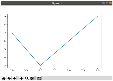
Matplotlib basic plot.
It’s important to note that plt.show() must be there in order for the graph to be displayed. This is the basics of plotting your first graph using Matplotlib, but there are a lot more nifty things that you can do with this graphing library. Matplotlib features are similar to MATLAB. It supports multiple windowing environments such as GTK, Tkinter, Qt, and wxWindows as well as several non-interactive backends like pdfs.
Let’s build on top of the example that we had before. Let’s say that you want to add a label to the x-axis. The code for doing this is listed below:
>>> plt.plot([5,6,7,8],[7,3,6,9])
[<matplotlib.lines.Line2D object at 0x7f4b772e3c50>]
>>> plt.xlabel("The X-Axis")
Text(0.5,0,'The X-Axis')
>>> plt.ylabel("The Y-Axis")
Text(0,0.5,'The Y-Axis')
>>> plt.show()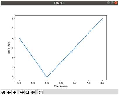
Matplotlib x-and-y axes labels.
As you can see in the updated graph the x and y axes now have labels. You can replace the text with any string you want. There are also more formatting options you can apply to the graph. For example, you can add an axis and a title. To add a title use plt.title() and to add an axis use plt.axis().
An example on how to use the plot() function to modify the plot is listed below:
>>> import matplotlib.pyplot as plt
>>> plt.plot([0,1,2,3,4],[3,6,9,12,15], "c*")
>>> plt.axis([0,10,0,20])
>>> plt.show()
The plot that’s displayed is listed below:
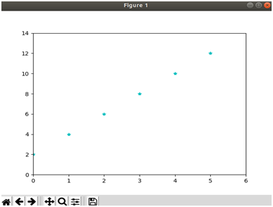
Using a Marker in Matplotlib.
As you can see from the code snippet the plot() function needs to be able to accept an unlimited number of arguments to adhere to the various types of plots. The number of elements in x must match the number of elements in y or less an error will occur. For example, the following will cause an issue:
>>> plt.plot([1,2,3],[2,4])Here’s what the error message say:
ValueError: x and y must have same first dimension, but have shapes (3,) and (2,)In order to fix this issue the length of both lists must be equal as corrected in the following coding snippet:
>>> plt.plot([1,2,3],[2,4,6])Also, if you’re confused about what "c*” stands for then just remember that these are optional parameters that control the line style or marker. The character 'c' represents the color cyan, and '*' is a star marker which means that there will be stars instead of points.
The following code shows how to create a sinusoidal plot:
>>> import matplotlib.pyplot as plt
>>> import numpy as np
>>> si = np.arange(0,100)
>>> plt.plot(np.sin(si))
>>> plt.show()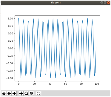
Sinusoidal waves plot.
Bar chart
There are many kinds of plots that you can create with Matplotlib such as bar, line, and pie charts. The below code plots a simple bar chart:
>>> import matplotlib.pyplot as plt
>>> import numpy as np
>>> x = np.arange(1,5) # ndarray of 1-4
>>> height = x ** 2  # square elements in x
>>> plt.bar(x, height, width = 0.35, align ="center", color ="green", edgecolor="black")
>>> plt.title("Bar Graph Demo")
>>> plt.show()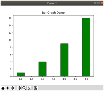
Bar Graph Demo.
Scatter plot
Below is the signature for a scatter plot in Python:
matplotlib.pyplot.scatter(x, y, s=None, c=None, marker=None, cmap=None, norm=None, vmin=None, vmax=None, alpha=None, linewidths=None, verts=None, edgecolors=None, hold=None, data=None, **kwargs)[source]Below is the code for a simple scatter plot:
>>> import matplotlib.pyplot as plt
>>> import numpy as np
>>> x = np.arange(1,51)
>>> y = np.random.rand(50)
>>> colors = np.random.rand(50)
>>> plt.scatter(x,y,c=colors)
>>> plt.show()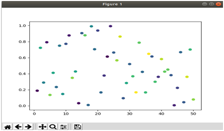
Scatter plot demo.
Coding Challenge*
Challenge 1: Matplotlib provides the ability to create shapes. Create a green circle with a .50 radius in Matplotlib.
Challenge 2: Plot a histogram that draws 500 random samples from a normal Gaussian distribution. The histogram should have a bin of 50, be green, and include a ylabel with the name Probability.
Challenge 3: Learn about 3D plotting in Matplotlib by reading the mplot3d tutorial. After reading the tutorial create a 3D line, bar, and scatter plot.