ejohnson643 / EMBEDR

Statistical quality evaluation of dimensionality reduction algorithms

EMBEDR

Author: Eric Johnson
Date Created: July 1, 2021
Email: [e-mail]

Overview

Empirical Marginal resampling Better Evaluates Dimensionality Reduction, or EMBEDR, is a method for evaluating the extent to which an embedding generated by a dimensionality reduction algorithm contains structures that are more similar to the structures in the high-dimensional space than we expect by random chance. The method applies the concept of an empirical hypothesis test, where a null distribution for a sample statistic is generated via marginal resampling, in order to estimate whether samples are better-embedded than a given DRA might do by chance.

For complete details, see our publication.

Installation

To install EMBEDR, we recommend cloning this repository before installing using pip in the main project directory. Specifically:

pip install .

The package requires numpy, scikit-learn, scipy, conda, and numba for installation. To generate figures, the seaborn package is required. Additionally, it is recommended that you ensure that fftw is installed, otherwise you will not be able to use the fast FIt-SNE implementation of the t-SNE algorithm. You can install fftw using homebrew.

Getting Started

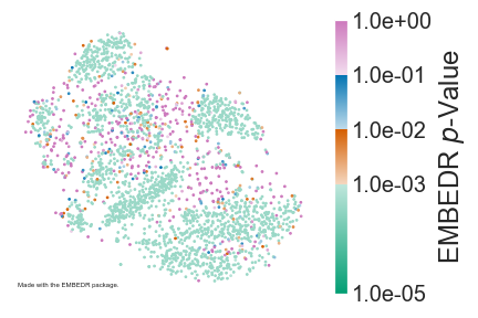
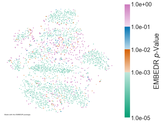
Once you've installed EMBEDR, you can easily generate an embedding colored by EMBEDR p-value by calling the fit method in the EMBEDR class as below.

from EMBEDR import EMBEDR, EMBEDR_sweep
import numpy as np

X = np.loadtxt("./data/mnist2500_X.txt").astype(float)

embObj = EMBEDR(project_dir='./')
embObj.fit(X)
embObj.plot()

In the example above, we embed 2500 MNIST digits once using t-SNE and we embed a marginally-resampled null data set once as well. The quality of the data embedding, based on the correspondence between the neighborhoods of each sample in the original space and the shown projection, are compared to those expected to be generated by signalless data (as generated by the null data set). This comparison results in a "p-value," which we use to color the samples in the embedding. For complete details, see our preprint.

The EMBEDR package primarily works through the EMBEDR class object, as in the example above. Importantly, because EMBEDR generates several embeddings of a data set (and a generated null data set), the method stores intermediate results in a project directory. In the example above, the project_dir variable is set to the current working directory, but we recommend that you set a specified "projects" directory. The default value for project_dir is ./projects/. To facilitate this organization, a project_name parameter can also be specified. If you don't want to do file caching, set do_cache=False when initializing the EMBEDR object.

Other useful parameters are:

• DRA: the dimensionality reduction algorithm; currently only tSNE and UMAP are supported.
• perplexity/nearest_neighbors: Set the algorithm hyperparameters for t-SNE or UMAP. Defaults are to set these at 10% of the number of samples.
• n_data_embed and n_null_embed: The number of data and null embeddings to generate before calculating EMBEDR p-values. Defaults are set at 1, but in practice using 3-10 embeddings is recommended. For a complete list of options, check the EMBEDR class documentation.

Performing a perplexity Sweep

Some of the most powerful results come from using EMBEDR to sweep across scales in the data by embedding data at several hyperparameter values. This is can be performed in this package using the EMBEDR_sweep class. This class wraps around the EMBEDR class to manage this parameter sweep. A simple example is shown below:

sweepObj = EMBEDR_sweep(project_name="EMBEDR_Sweep_Example",
                        project_dir="./projects/",
                        DRA='tsne',
                        n_jobs=-1,  ## Set to -1 to use all available processors.
                        verbose=3,  ## Set to 0 to suppress output.
                        n_data_embed=3,
                        n_null_embed=1,
                        sweep_type='perplexity',
                        sweep_values=[25, 100, 250])
sweepObj.fit(X)
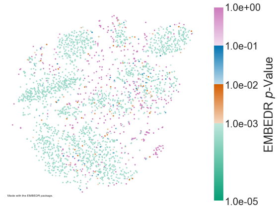
sweepObj.plot_embedding(embed_2_show=1, param_2_plot=250)

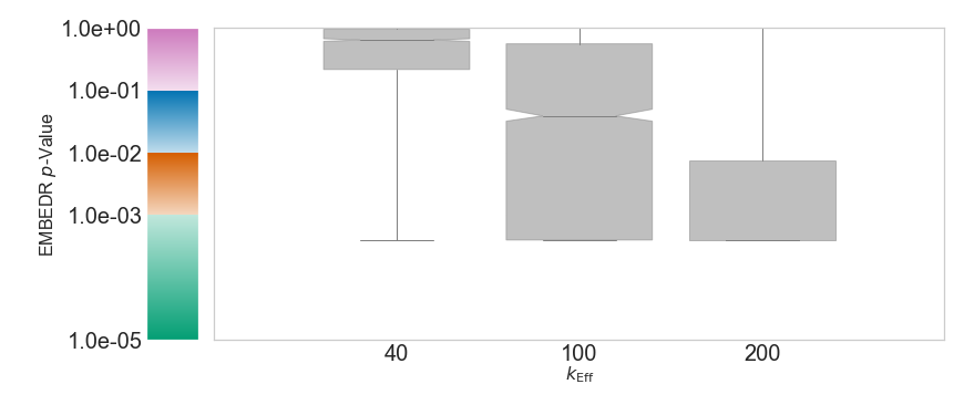
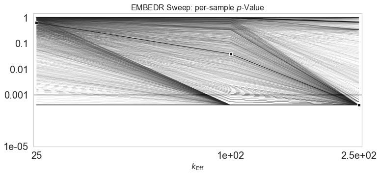
In this example, at perplexity = 25, 100, and 250, we embedded the data 3 times, each with a different random initialization, and we embedded the null data once. We can then plot any of the embeddings at any of the values of perplexity using the plot_embedding method shown above. We can also visualize the entire sweep using the sweep_boxplot and sweep_lineplot functions, as shown below.

sweepObj.sweep_boxplot()
sweepObj.sweep_lineplot()

Using these figures, we can summarize the quality of t-SNE as the perplexity hyperparameter is varied. Using these figures, as shown in our paper, we can determine optimal values for perplexity (or n_neighbors in UMAP), find characteristic scales and neighborhood sizes for different samples, and detect robust features in embeddings. We can also determine the optimal perplexity for each sample individually and use this perplexity to generate a sample-wise optimal embedding of the data. This is again faciliated by the EMBEDR_sweep class method fit_samplewise_optimal. After calling this method, using the plot_embedding method with the EMBEDR_sweep class will show this sample-wise optimal embedding. This process can only be carried out after a sweep has been run. Additionally, the optimal perplexity values will only be selected from those used int he sweep.

sweepObj.fit_samplewise_optimal()
sweepObj.plot_embedding()

To generate more embeddings or run a sweep with different hyperparameter values, the EMBEDR or EMBEDR_sweep classes can be reinitialized and fitted again. If file caching is permitted, then the package will first look for previously generated embeddings that match the set parameters. This means that making small changes to runs will not waste previous work. For example, if we change n_data_embed to 5 after running the previous example, only 2 new embeddings will be generated for each value of perplexity because 3 have already be generated. The EMBEDR package also uses this process to avoid recalculating nearest neighbor graphs and affinity matrices.

New in Version 2.0

The updated version of the EMBEDR package better facilitates the EMBEDR algorithm as described in our manuscript by improving the flow of data between stages of the algorithm. In particular, we greatly reduce the number of times that kNN graphs and affinity matrices are calculated; attemping to re-use calculations as often as possible.

This version of the algorithm also supports the sample-wise specification of the perplexity and n_neighbors parameters, which are common hyperparameters for dimensionality reduction algorithms.

The EMBEDR_sweep object has been implemented. Users can now execute a sweep over perplexity or n_neighbors. Users can also fit a cell-wise optimal t-SNE embedding as in Figure 7 of the manuscript.

New in Version 2.1

The method now supports UMAP, although not to the same level as t-SNE. It seems that UMAP will soon be supporting the use of pre-computed kNN graphs, at which point UMAP and t-SNE will be able to be used interchangably.

A bug where EMBEDR objects could only be reloaded from the original path at which they were created has been amended and will be backwards compatible with previous versions. Objects can now be loaded from any relative path specification for the project directory.