This is a data analysis for my Clash Royale Season 35 battles, as a log bait player (except for one X-Bow battle by mistake). The goals of the current analysis are:
Part I: Exploratory Data Analysis:
- Explore patterns of win/defeat and investigate my own win rate of the current season.
- Investigate the trophy change distribution (+ve/-ve) after each battle.
- Explore patterns of win/defeat streaks.
- Finding out the most common cards in my opponents decks.
Part II: Inference:
- Build a Bayesian model to infer distributions for: win rate, positive trophy change and negative trophy change.
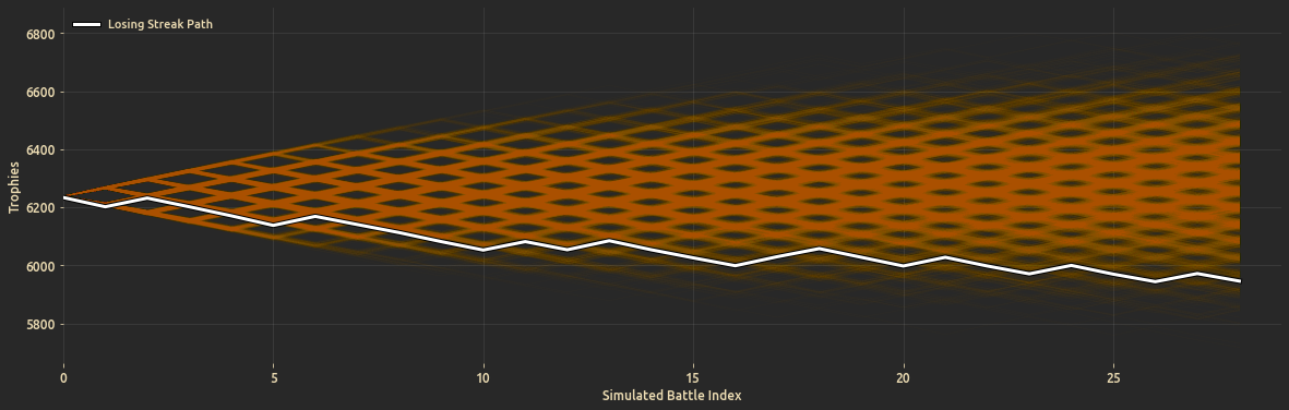
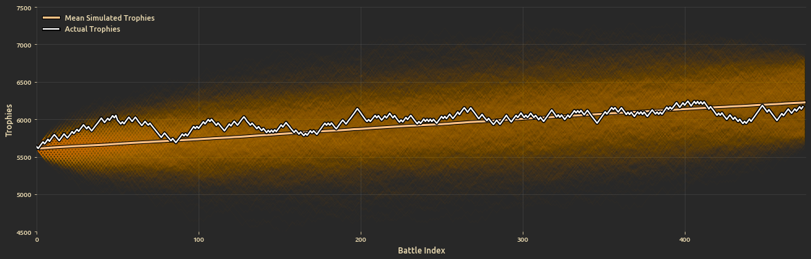
- Simulate random walk battles to compare actual progression vs. the simulated battles.
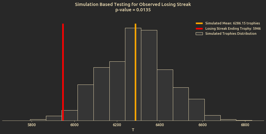
- Test a particular observed lose streak and calculate the probability of its occurence by simulating a random battle walks.
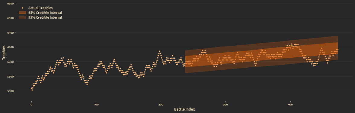
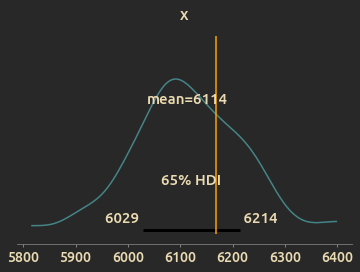
- Build a Bayesian linear regression model to predict the season ending trophies.
Data have been collected on a daily basis using miner.py, and in data.csv we have 474 battles, with the following summary statistics:
Season Starting Trophies = 5609 trophies
Season Ending Trophies = 6168 trophies
Overall Observed Win rate = 51.27%
Total Trophy Change since season start = 650 trophies
Total number of battles = 474 battles
Active playing days = 32 days
Avg. rate of trophy increase = 20.31 trophies/day
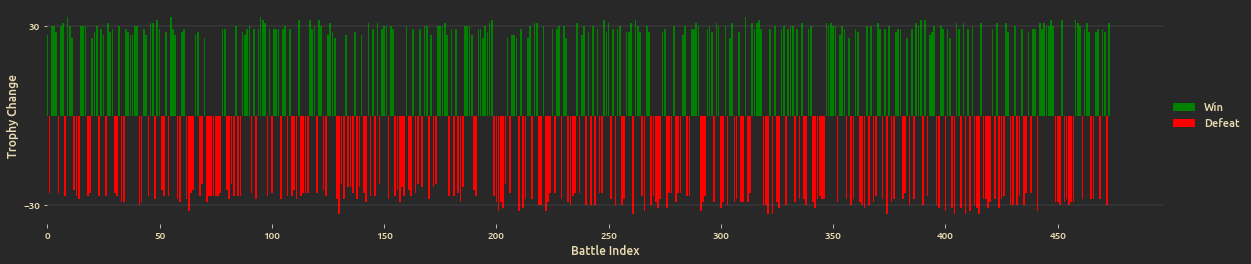
Let's visualize battles outcome (win/defeat), coupled with trophy gain/loss:
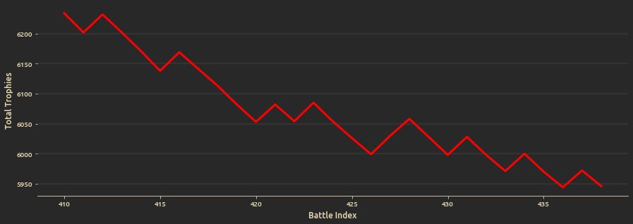
And progression of trophies since season start until the final battle:

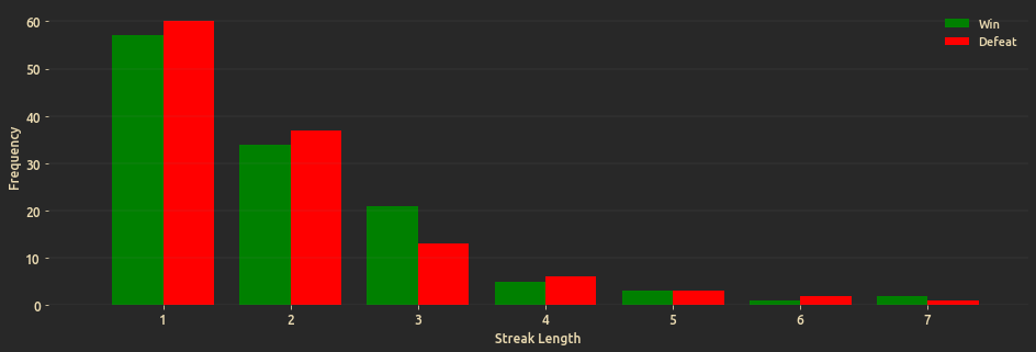
How often did win/defeat streaks occur?
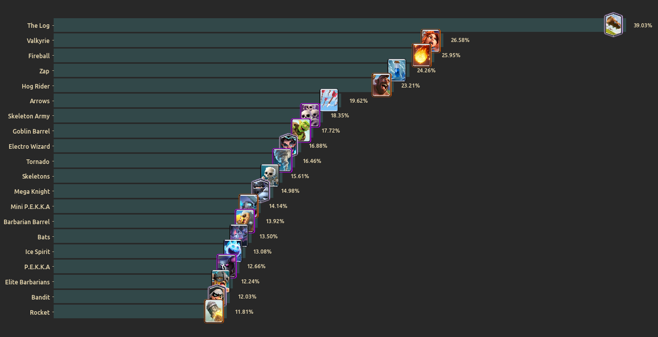
What are our opponents most common cards?
Note: this does not sum to 100% because one opponent can have a mix of most common card in their deck, the following plot shows the percentage of having a specific card in all decks I have faced.
We don't treat the win rate as just the observed fixed value, but as a random variable. We assume that our data
Prior:
Likelihood:
Posterior:
Win rate trace plot:
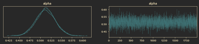
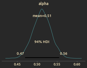
Posterior distribution of win rate
How much trophies do we expect to win/lose after each battle? to answer this we model the observed trophy change (27, 29, 29, 30, .., 33) as a Categorical distribution with a Drichlet prior, for both the positive and negative change.
Prior:
Likelihood:
Trace plots for
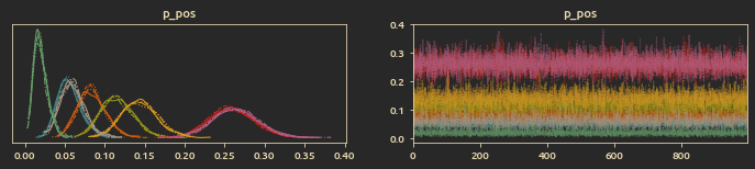
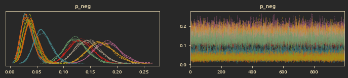
Distribution plot of positive and negative trophy change (at posterior mean values):
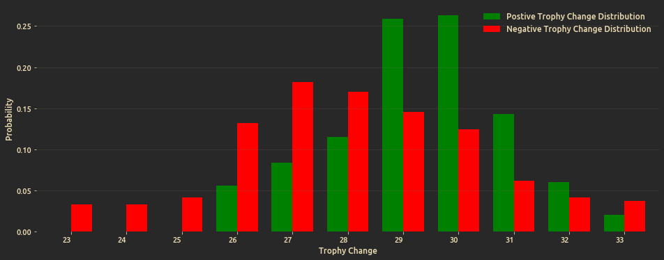
One can conclude that for me the game was on average more rewarding than it was punishing. I was able to win more trophies than I lost, mode of positive trophy change is 30 while for negative trophy change it's 27, so despite the low win rate, the game on average is rewarding.
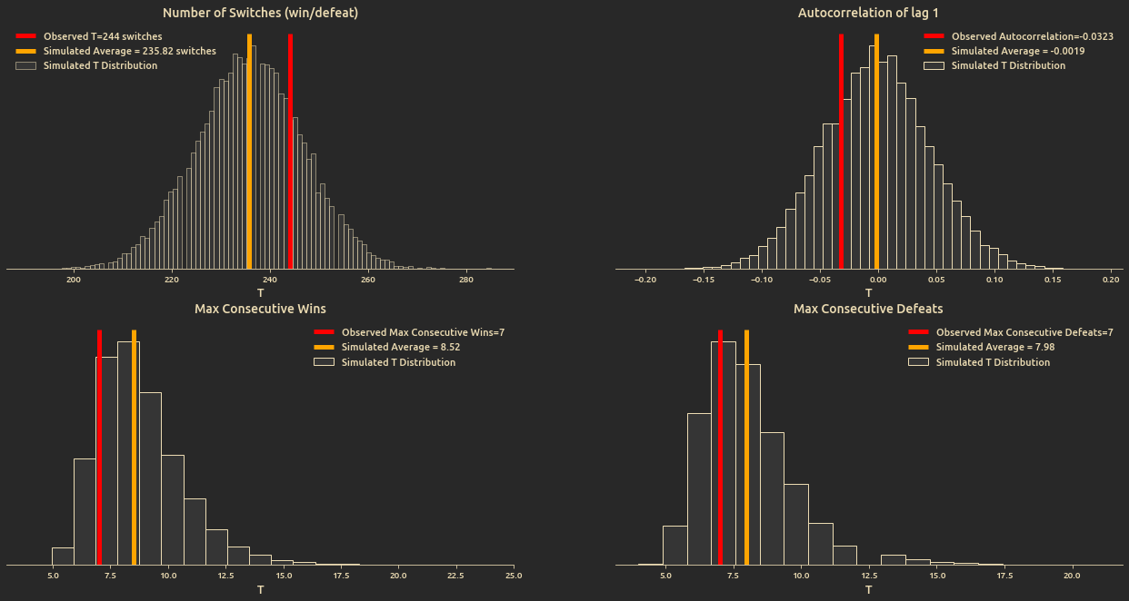
I don't think each battle outcome is independent, but if we proceeded anyway to assume that, and given the data we have, is this a valid assumption? In order to test this we define a 4 Test statistics:
- The number of switches between wins and defeats.
- Autocorrelation of lag 1
- Maximum consecutive wins (consecutive ones)
- Maximum consecutive defeats (consecutive zeroes)
We draw large enough samples from posterior predictive distribution and find the distribution of each test statistic
Yet, we found no significant difference from the mean:
TODO: Add model formulation, results and summary
TODO: Add model formulation, results and summary
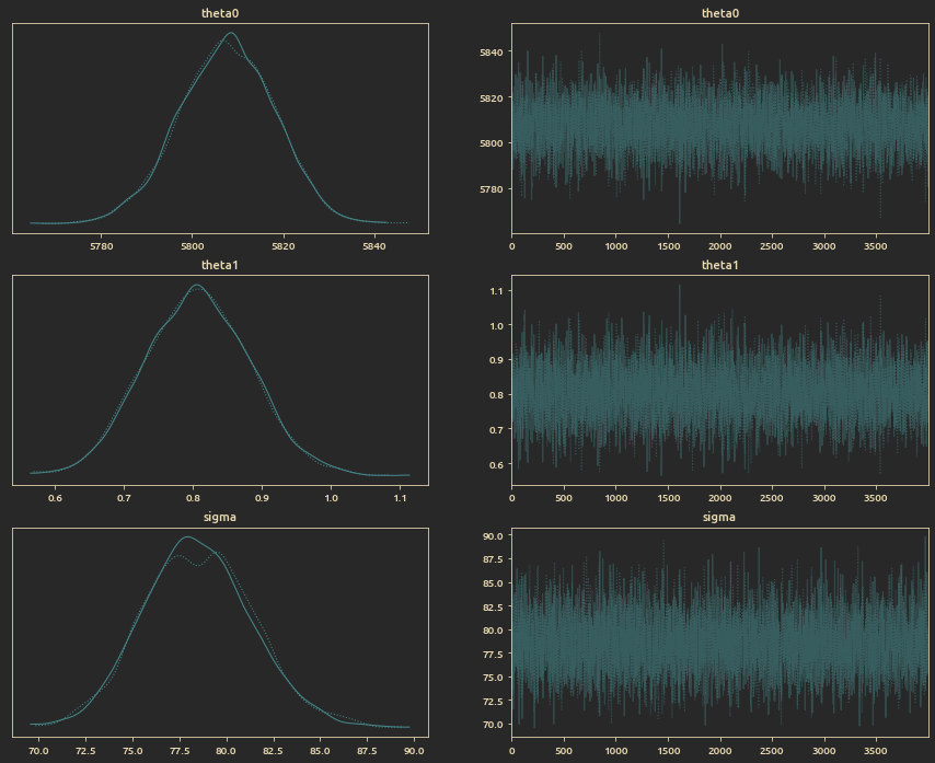
Linear regression model parameters trace plot:
TODO: Explain the need for this and add model forumlation, results and summary.