SolarSpec group script for fitting XPS data using a Shirley background
Explore the docs »
View Demo
·
Report Bug
·
Request Feature
Table of Contents
 Fitting XPS data using a Shirley background
To begin using this app is very simple. Just verify you have the necessary prequisites and follow the installation instructions.
Make sure MATLAB is installed. It is available for download in the Software Distribution section under the Help tab after you log into Canvas. Click on the "Add-Ons" dropdown menu of your MATLAB Home screen. Then click on "Manage Add-Ons" and ensure you have the Image Processing Toolbox and the Signal Processing Toolbox. If not, click on the "Get Add-Ons" button instead and search for the aforementioned products.
-
Clone the repo to your PC
git clone https://github.com/SolarSpec/TaucPlotGUI.git
-
Now enter the repository and install the application in MATLAB
Click on the .mlappinstall file in your repository -
Browse the APPS header and click on the drop down.
You will find the recently installed application under 'MY APPS' and can add it to your favourites
XPS is a technique using high energy light (X-rays) to eject electrons from a material. If one knows the energy of the X-ray, then on can determine how strongly the the released electron is bound to the core of the material. The fitted peaks tell the user about the center and relative energies of the material which can describe how many unique atoms are present in said material.
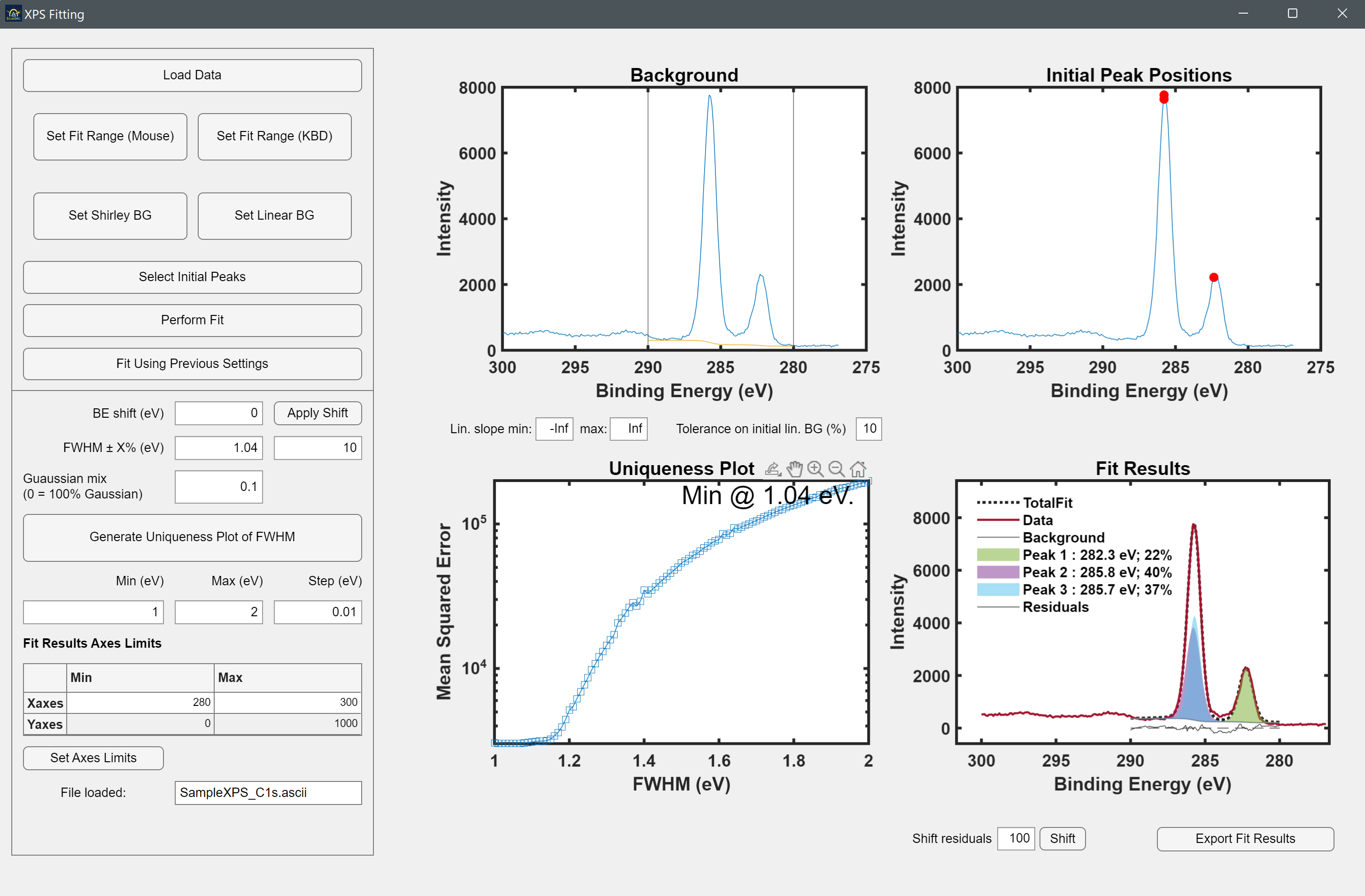
Begin by loading some XPS data in the form of an .ascii file. The user can either set the fit range by mouse or by keyboard (KBD) input using the respective "Set Fit Range" buttons, which will draw xlines on the specified x-coordinates. Next is to choose the type of background to set, either "Shirley BG" or "Linear BG" using the respective buttons which will actively iterate to find the Shirley Background or you can draw an ROI line between the ends of the peak regions for the Linear Background. The three edit fields below the Background axes allow the user to manually input the minimum and maximum values of the Linear background line and the tolerance value determines how much the slope change from the initial endpoints.
Next the user can click the "Select Initial Peaks" button to approximate the initial peaks of the loaded data by clicking the cursor on the "Initial Peak Positions" axes. When complete, the user can press enter to continue. Next determine the Full Width Half Max value (FWHM) by clicking on the "Generate Uniqueness Plot of FWHM" button, which uses a mix of Gaussian and Lorentz distributions (this app uses sum of each distribution instead of the product). The FWHM can also be constrained to a default value of +- 10% or any inputted percentage.
The Uniqueness plot generates the fit for all the FWHM values with the bounds and step inbetween. It outputs the Mean Squared Error (MSE) vs FWHM. The user can see where the fitting is best with the least amount of error and has the desired value outputted on the plot itself. Next, with this minimum error FWHM value, the user can enter this value back into the "FWHM +- X%" field and click the "Perform Fit" button for the best looking Fit Result plot.
After clicking "Perform Fit", the GUI gives the peak center and relative areas in percentage. Change the axes limits from the bottom left table, which only affects the Fit Result plot. The residuals are also plotted beneath the fit where the dashed line is effectively zero and the solid line is the difference between the original data and the calculated fit. You can shift it this object on the plot by editing the value beneath the Fit Results plot and clicking the "Shift" button. Export the fit results in the folder where the data was grabbed; the button returns a fit parameters file and an .emf figure of the Fit Result plot. The user can fit using previous settings if you open new but similar data by clicking the "Fit Using Previous Settings" button. This button saves the Fit Range bounds as well as the Inital Peak guesses and then reruns the same functions as before.
This app is currently lacking in any examples to be shown as it is still being created
For more information on any of the internal functions, please refer to the MATLAB Documentation
- Plot XPS Intensity vs. Binding Energy (eV)
- Use the cursor to approximate initial peak positions
- Set the fit range by keyboard or mouse input
- Set either a Shirley or Linear background
- Generate a Uniqueness Plot to determine the best FWHM value
- Perform a Fit Results
- View residuals of data below results
See the open issues for a full list of proposed features (and known issues).
Contributions are what make the open source community such an amazing place to learn, inspire, and create. Any contributions you make are greatly appreciated.
If you have a suggestion that would make this better, please fork the repo and create a pull request. You can also simply open an issue with the tag "enhancement". Don't forget to give the project a star! Thanks again!
- Fork the Project
- Create your Feature Branch (
git checkout -b feature/AmazingFeature) - Commit your Changes (
git commit -m 'Add some AmazingFeature') - Push to the Branch (
git push origin feature/AmazingFeature) - Open a Pull Request
Distributed under the BSD 3-Clause License. See LICENSE.txt for more information.
SolarSpec - SolarSpec Website - vidihari@student.ubc.ca
Project Link: https://github.com/SolarSpec/XPSfitting