Flow Shop Scheduling

Job shop scheduling (JSS) is an optimization problem with the goal of scheduling, on a number of machines, jobs with diverse orderings of processing on the machines. The objective is to minimize the schedule length, also called "makespan," or completion time of the last task of all jobs. Flow shop scheduling (FSS) is a constrained case of JSS where every job uses every machine in the same order. The machines in FSS problems can often be seen as sequential operations to be executed on each job, as is the case in this particular demo.

This example demonstrates three ways of formulating and optimizing FSS:

Formulating a nonlinear model and solving on a Leap hybrid nonlinear-model solver
Formulating a constrained quadratic model (CQM) and solving on a Leap hybrid CQM solver
Formulating a mixed-integer problem and solving on a classical mixed-integer linear solver

This example lets you run the scheduler from either the command line or a visual interface built with Dash.

Usage

Your development environment should be configured to access Leap’s Solvers. You can see information about supported IDEs and authorizing access to your Leap account here.

To run the flow shop demo with the visual interface, from the command line enter

python app.py

Access the user interface with your browser at http://127.0.0.1:8050/.

To run the flow shop scheduler without the Dash interface, from the command line enter

python job_shop_scheduler.py [-h] [-i INSTANCE] [-tl TIME_LIMIT] [-os OUTPUT_SOLUTION] [-op OUTPUT_PLOT] [-m] [-v] [-q] [-p PROFILE] [-mm MAX_MAKESPAN]

This calls the FSS algorithm for the input file. Command line arguments are as follows:

-h (or --help): show this help message and exit
-i (--instance): path to the input instance file (default: input/tai20_5.txt); see app_configs.py for instance names
-tl (--time_limit) time limit in seconds (default: None)
-os (--output_solution): path to the output solution file (default: output/solution.txt)
-op (--output_plot): path to the output plot file (default: output/schedule.png)
-m (--use_scipy_solver): use SciPy's HiGHS solver instead of the CQM solver (default: True)
-m (--use_nl_solver): use the nonlinear-model solver instead of the CQM solver (default: False)
-v (--verbose): print verbose output (default: True)
-p (--profile): profile variable to pass to the sampler (default: None)
-mm (--max_makespan): manually set an upper-bound on the schedule length instead of auto-calculating (default: None)

Problem Instances

Several problem instances are pre-populated under the input folder. Some of these instances are contained within the flowshop1.txt file, retrieved from the OR-Library, and parsed when the demo is initialized. These can be accessed as if they were files in the input folder, named according to the instance short names in flowshop1.txt (e.g., "car2", "reC13"), without filename endings. Other instances were pulled from E. Taillard's list of benchmarking instances. If the string "tai" is in the filename, the model expects the format used by Taillard.

Model and Code Overview

Problem Parameters

These are the parameters of the problem:

n: the number of jobs
m: the number of machines
J: set of jobs ({0,1,2,...,n-1})
M: set of machines ({0,1,2,...,m-1})
T: set of tasks ({0,1,2,...,m-1}) that has same dimension as M
M_(j,t): the machine that processes task t of job j
T_(j,i): the task that is processed by machine i for job j
D_(j,t): the processing duration that task t needs for job j
V: maximum possible makespan

Variables

w: a positive integer variable that defines the completion time (makespan) of the JSS
x_(j_i): positive integer variables used to model start of each job j on machine i
y_(j_k,i): binaries which define if job k precedes job j on machine i

Objective

The objective is to minimize the makespan (w) of the given FSS problem.

Nonlinear Model

The nonlinear model represents the problem using only the job order for the machines. This is sufficient to construct feasible, compact solutions. In seeking a minimum, the model uses Ocean's dwave-optimization package's ListVariable to efficiently permutate the order of jobs.

Typically, solver performance strongly depends on the size of the solution space for the modeled problem: models with smaller spaces of feasible solutions tend to perform better than ones with larger spaces. A powerful way to reduce the feasible-solutions space is by using variables that act as implicit constraints, such as the ListVariable symbol used here, where the order of jobs is a permutation of values. The max operation is used to extract the start time for each job, making sure that there's no overlap between jobs on machines. No other constraints are necessary.

As can be seen in the two example images below, switching the job order can improve the solution quality, corresponding to a lowering of the completion time, or the makespan, for the FSS problem.

Above: a solution to a flow shop scheduling problem with 3 jobs on 3 machines.

Above: an improved solution to the same problem with a permutated job order.

Constrained Quadratic Model

The constrained quadratic model (CQM) requires adding a set of constraints to ensure that tasks are executed in order and that no single machine is used by different jobs at the same time.

Precedence Constraint

Our first constraint, equation 1, enforces the precedence constraint. This ensures that all tasks of a job are executed in the given order.

(1)

This constraint ensures that a task for a given job, j, on a machine, M_(j,t), starts when the previous task is finished. As an example, for consecutive tasks 4 and 5 of job 3 that run on machine 6 and 1, respectively, assuming that task 4 takes 12 hours to finish, we add this constraint: x_3_6 >= x_3_1 + 12

No-Overlap Constraints

Our second constraint, equation 2, ensures that multiple jobs don't use any machine at the same time. (2)

Usually this constraint is modeled as two disjunctive linear constraints (Ku et al. 2016 and Manne et al. 1960); however, it is more efficient to model this as a single quadratic inequality constraint. In addition, using this quadratic equation eliminates the need for using the so called Big M value to activate or relax constraint (https://en.wikipedia.org/wiki/Big_M_method).

The proposed quadratic equation fulfills the same behaviour as the linear constraints:

There are two cases:

if y_j,k,i = 0 job j is processed after job k: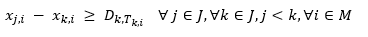
if y_j,k,i = 1 job k is processed after job j: Since these equations are applied to every pair of jobs, they guarantee that the jobs don't overlap on a machine.

Makespan Constraint

In this demonstration, the maximum makespan can be defined by the user or it will be determined using a greedy heuristic. Placing an upper bound on the makespan improves the performance of the D-Wave sampler; however, if the upper bound is too low then the sampler may fail to find a feasible solution.

References

A. S. Manne, On the job-shop scheduling problem, Operations Research , 1960, Pages 219-223.

Wen-Yang Ku, J. Christopher Beck, Mixed Integer Programming models for job shop scheduling: A computational analysis, Computers & Operations Research, Volume 73, 2016, Pages 165-173.

License

Released under the Apache License 2.0. See LICENSE file.

dwave-examples / flow-shop-scheduling