dseo23 / dsc-tuning-neural-networks-with-normalization

Tuning Neural Networks with Normalization

Introduction

Now that we've investigated some methods for tuning our networks, we will investigate some further methods and concepts regarding reducing training time. These concepts will begin to form a more cohesive framework for choices along the modeling process.

Objectives

You will be able to:

• Explain what normalization does to training time with neural networks and why
• Explain what a vanishing or exploding gradient is, and how it is related to model convergence
• Compare the different optimizer strategies for neural networks

Normalized Inputs: Speed up Training

One way to speed up training of your neural networks is to normalize the input. In fact, even if training time were not a concern, normalization to a consistent scale (typically 0 to 1) across features should be used to ensure that the process converges to a stable solution. Similar to some of our previous work in training models, one general process for standardizing our data is subtracting the mean and dividing by the standard deviation.

Vanishing or Exploding Gradients

Not only will normalizing your inputs speed up training, it can also mitigate other risks inherent in training neural networks. For example, in a neural network, having input of various ranges can lead to difficult numerical problems when the algorithm goes to compute gradients during forward and back propagation. This can lead to untenable solutions and will prevent the algorithm from converging to a solution. In short, make sure you normalize your data! Here's a little more mathematical background:

To demonstrate, imagine a very deep neural network. Assume $g(z)=z$ (so no transformation, just a linear activation function), and biases equal to 0.

$\hat y = w^{[L]}w^{[L-1]}w^{[L-2]}... w^{[3]}w^{[2]}w^{[1]}x$

recall that $z^{[1]} =w^{[1]}x $, and that $a^{[1]}=g(z^{[1]})=z^{[1]}$

similarly, $a^{[2]}=g(z^{[2]})=g(w^{[2]}a^{[1]})$

Imagine two nodes in each layer,

Even if the $w$'s are slightly smaller than 1 or slightly larger, the activations will explode when there are many layers in the network!

Other Solutions to Vanishing and Exploding Gradients

Aside from normalizing the data, you can also investigate the impact of changing the initialization parameters when you first launch the gradient descent algorithm.

For initialization, the more input features feeding into layer l, the smaller you want each $w_i$ to be.

A common rule of thumb is:

$Var(w_i) = 1/n $

or

$Var(w_i) = 2/n$

One common initialization strategy for the relu activation function is:

w^{[l]} = np.random.randn(shape)*np.sqrt(2/n_(l-1)) 

Later, we'll discuss other initialization strategies pertinent to other activation functions.

Optimization

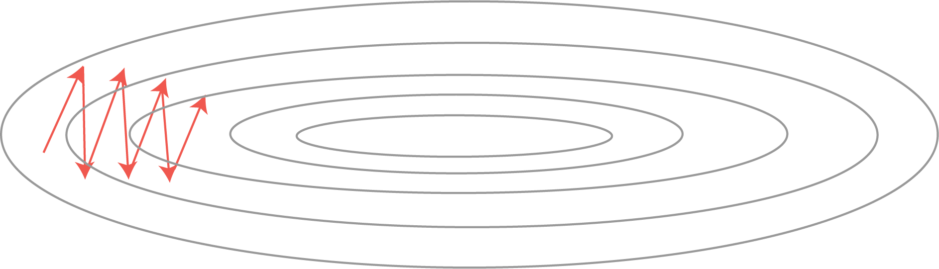
In addition, you could even use an alternative convergence algorithm instead of gradient descent. One issue with gradient descent is that it oscillates to a fairly big extent, because the derivative is bigger in the vertical direction.

With that, here are some optimization algorithms that work faster than gradient descent:

Gradient Descent with Momentum

Compute an exponentially weighted average of the gradients and use that gradient instead. The intuitive interpretation is that this will successively dampen oscillations, improving convergence.

Momentum:

• compute $dW$ and $db$ on the current minibatch

• compute $V_{dw} = \beta V_{dw} + (1-\beta)dW$ and

• compute $V_{db} = \beta V_{db} + (1-\beta)db$

These are the moving averages for the derivatives of $W$ and $b$

$W:= W- \alpha Vdw$

$b:= b- \alpha Vdb$

This averages out gradient descent, and will "dampen" oscillations. Generally, $\beta=0.9$ is a good hyperparameter value.

RMSprop

RMSprop stands for "root mean square" prop. It slows down learning in one direction and speed up in another one. On each iteration, it uses exponentially weighted average of the squares of the derivatives.

$S_{dw} = \beta S_{dw} + (1-\beta)dW^2$

$S_{db} = \beta S_{dw} + (1-\beta)db^2$

$W:= W- \alpha \dfrac{dw}{\sqrt{S_{dw}}}$ and

$b:= b- \alpha \dfrac{db}{\sqrt{S_{db}}}$

In the direction where we want to learn fast, the corresponding $S$ will be small, so dividing by a small number. On the other hand, in the direction where we will want to learn slow, the corresponding $S$ will be relatively large, and updates will be smaller.

Often, add small $\epsilon$ in the denominator to make sure that you don't end up dividing by 0.

Adam Optimization Algorithm

"Adaptive Moment Estimation", basically using the first and second moment estimations. Works very well in many situations! It takes momentum and RMSprop to put it together!

Initialize:

$V_{dw}=0, S_{dw}=0, V_{db}=0, S_{db}=0$

For each iteration:

Compute $dW, db$ using the current mini-batch:

$V_{dw} = \beta_1 V_{dw} + (1-\beta_1)dW$, $V_{db} = \beta_1 V_{db} + (1-\beta_1)db$

$S_{dw} = \beta_2 S_{dw} + (1-\beta_2)dW^2$, $S_{db} = \beta_2 S_{db} + (1-\beta_2)db^2$

It's like momentum and then RMSprop. We need to perform a correction! This is sometimes also done in RSMprop, but definitely here too.

$$V^\mathbf{corr}_{dw}= \dfrac{V_{dw}}{1-\beta_1^t}, V^{corr}_{db}= \dfrac{V_{db}}{1-\beta_1^t}$$ $$S^{corr}_{dw}= \dfrac{S_{dw}}{1-\beta_2^t}, S^{corr}_{db}= \dfrac{S_{db}}{1-\beta_2^t}$$ $$W:= W- \alpha \dfrac{V^{corr}_{dw}}{\sqrt{S^{corr}_{dw}+\epsilon}} \text{ and } b:= b- \alpha \dfrac{V^{corr}_{db}}{\sqrt{S^{corr}_{db}+\epsilon}}$$

Hyperparameters:

• $\alpha$
• $\beta_1 = 0.9$
• $\beta_2 = 0.999$
• $\epsilon = 10^{-8}$

Generally, only $\alpha$ gets tuned.

Learning Rate Decay

Learning rate decreases across epochs.

$$\alpha = \dfrac{1}{1+\text{decay rate * epoch nb}}* \alpha_0$$

other methods:

$$\alpha = 0.97 ^{\text{epoch nb}}* \alpha_0$$

(or exponential decay)

or

$$\alpha = \dfrac{k}{\sqrt{\text{epoch nb}}}* \alpha_0$$

or

Manual decay!

Hyperparameter Tuning

Now that you've seen some optimization algorithms, take another look at all the hyperparameters that need tuning:

Most important:

• $\alpha$

Next:

• $\beta$ (momentum)
• Number of hidden units
• mini-batch-size

Finally:

• Number of layers
• Learning rate decay

Almost never tuned:

• $\beta_1$, $\beta_2$, $\epsilon$ (Adam)

Things to do:

• Don't use a grid, because hard to say in advance which hyperparameters will be important

Additional Resources

• https://www.coursera.org/learn/deep-neural-network/lecture/lXv6U/normalizing-inputs
• https://www.coursera.org/learn/deep-neural-network/lecture/y0m1f/gradient-descent-with-momentum

Summary

In this lesson you began learning about issues regarding the convergence of neural networks training. This included the need for normalization as well as initialization parameters and some optimization algorithms. In the upcoming lab, you'll further investigate these ideas in practice and observe their impacts from various perspectives.