dseo23 / dsc-confusion-matrices

Confusion Matrices

Introduction

In this lesson, you'll learn how to construct and interpret a Confusion Matrix to evaluate the performance of a classifier!

Objectives

You will be able to:

• Describe the four quadrants of a confusion matrix
• Interpret a confusion matrix
• Create a confusion matrix using scikit-learn

How to evaluate classifier performance?

A confusion matrix tells us four important things. Let's assume a model was trained for a Binary Classification task, meaning that every item in the dataset has a ground-truth value of 1 or 0. To make it easier to understand, let's pretend this model is trying to predict whether or not someone has a disease. A confusion matrix gives you the following information:

True Positives (TP): The number of observations where the model predicted the person has the disease (1), and they actually do have the disease (1).

True Negatives (TN): The number of observations where the model predicted the person is healthy (0), and they are actually healthy (0).

False Positives (FP): The number of observations where the model predicted the person has the disease (1), but they are actually healthy (0).

False Negatives (FN): The number of observations where the model predicted the person is healthy (0), but they actually have the disease (1).

Let's take a look at an example confusion matrix:

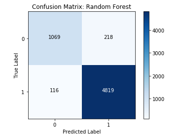
As you can see, one axis of the confusion matrix represents the ground-truth value of the items the model made predictions on, while the other axis represents the labels predicted by the classifier. To read a confusion matrix, look at the intersection of each row and column to tell what each cell represents. For instance, in the example above, the bottom right square represents True Positives, because it is the intersection of "True Label: 1" row and the "Predicted Label: 1" column.

Take another look at the diagram above and see if you can figure out which cells represent TN, FP, and FN.

Confusion matrices for multi-categorical classification

So far, we've kept it simple by only focusing on confusion matrices for binary classification problems. However, it's common to see classification tasks that are multi-categorical in nature. We can keep track of these by just expanding the number of rows and columns in our confusion matrix!

This example is from the Reuters Newsgroups dataset. As we can see in the example above, we use an equivalent number of rows and columns, with each row and column sharing the same index referring to the same class. In this, the true labels are represented by the rows, while the predicted classes are represented by the columns.

Take a look at the diagonal starting in the top-left and moving down to the right. This diagonal represents our True Positives since the indexes are the same for both row and column. For instance, we can see at location [19, 19] that 281 political articles about guns were correctly classified as political articles about guns. Since our model is multi-categorical, we may also be interested in exactly how a model was incorrect with certain predictions. For instance, by looking at [4, 19], you can conclude that 33 articles that were of category talk.politics.misc were incorrectly classified as talk.politics.guns. Note that when viewed through the lens of the talk.politics.misc, these are False Negatives -- our model said they weren't about this topic, and they were. However, they are also False Positives for talk.politics.guns, since our model said they were about this, and they weren't!

Use sklearn to create confusion matrices

Since confusion matrices are a vital part of evaluating supervised learning classification problems, it's only natural that sklearn has a quick and easy way to create them. You'll find the confusion_matrix() function inside the sklearn.metrics module. This function expects two arguments -- the labels, and the predictions, in that order.

from sklearn.metrics import confusion_matrix
example_labels = [0, 1, 1, 1, 0, 1, 0, 1, 0, 0, 1]
example_preds  = [0, 1, 0, 1, 0, 0, 1, 1, 1, 1, 1]

cf = confusion_matrix(example_labels, example_preds)
cf

array([[2, 3],
       [2, 4]])

One nice thing about using sklearn's implementation of a confusion matrix is that it automatically adjusts to the number of categories present in the labels. For example:

ex2_labels = [0, 1, 2, 2, 3, 1, 0, 2, 1, 2, 3, 3, 1, 0]
ex2_preds =  [0, 1, 1, 2, 3, 3, 2, 2, 1, 2, 3, 0, 2, 0]

cf2 = confusion_matrix(ex2_labels, ex2_preds)
cf2

array([[2, 0, 1, 0],
       [0, 2, 1, 1],
       [0, 1, 3, 0],
       [1, 0, 0, 2]])

Take a minute to examine the output above, and see if you can interpret the confusion matrix correctly. For instance, see if you can figure out how many 3's were mistakenly predicted to be a 0.

Summary

Confusion matrices are a very handy tool to help us quickly understand how well a classification model is performing. However, you'll see that the truly useful information comes when you use confusion matrices to calculate Evaluation Metrics such as accuracy, precision, and recall!