Introduction

Non-Intrusive Load Monitoring (NILM), also known as energy disaggregation, is a technology used to analyze and identify the energy consumption of individual appliances within a household or building without the need for dedicated sensors on each device. Instead, NILM relies on analyzing the overall electrical signal of the entire home or building to disaggregate and identify the specific energy consumption patterns of different appliances. The process involves using advanced signal processing and machine learning algorithms to distinguish the unique electrical signatures of various devices. By understanding the power consumption patterns associated with specific appliances, NILM systems can provide insights into how energy is being used, enabling homeowners and businesses to make informed decisions about energy efficiency, conservation, and management. This technology plays a crucial role in promoting energy awareness, optimizing energy usage, and ultimately contributing to more sustainable and cost-effective energy practices. The architecture on household-, bus-, and metering-level is illustrated below:

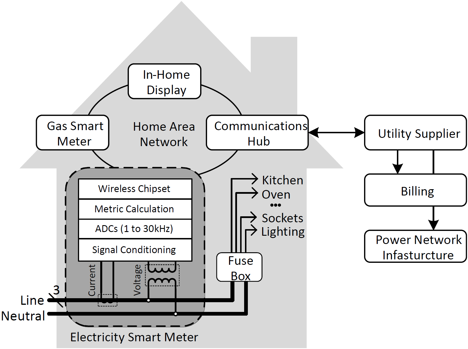Figure 1: Household level NILM architecture.

Figure 2: Bus level NILM architecture.

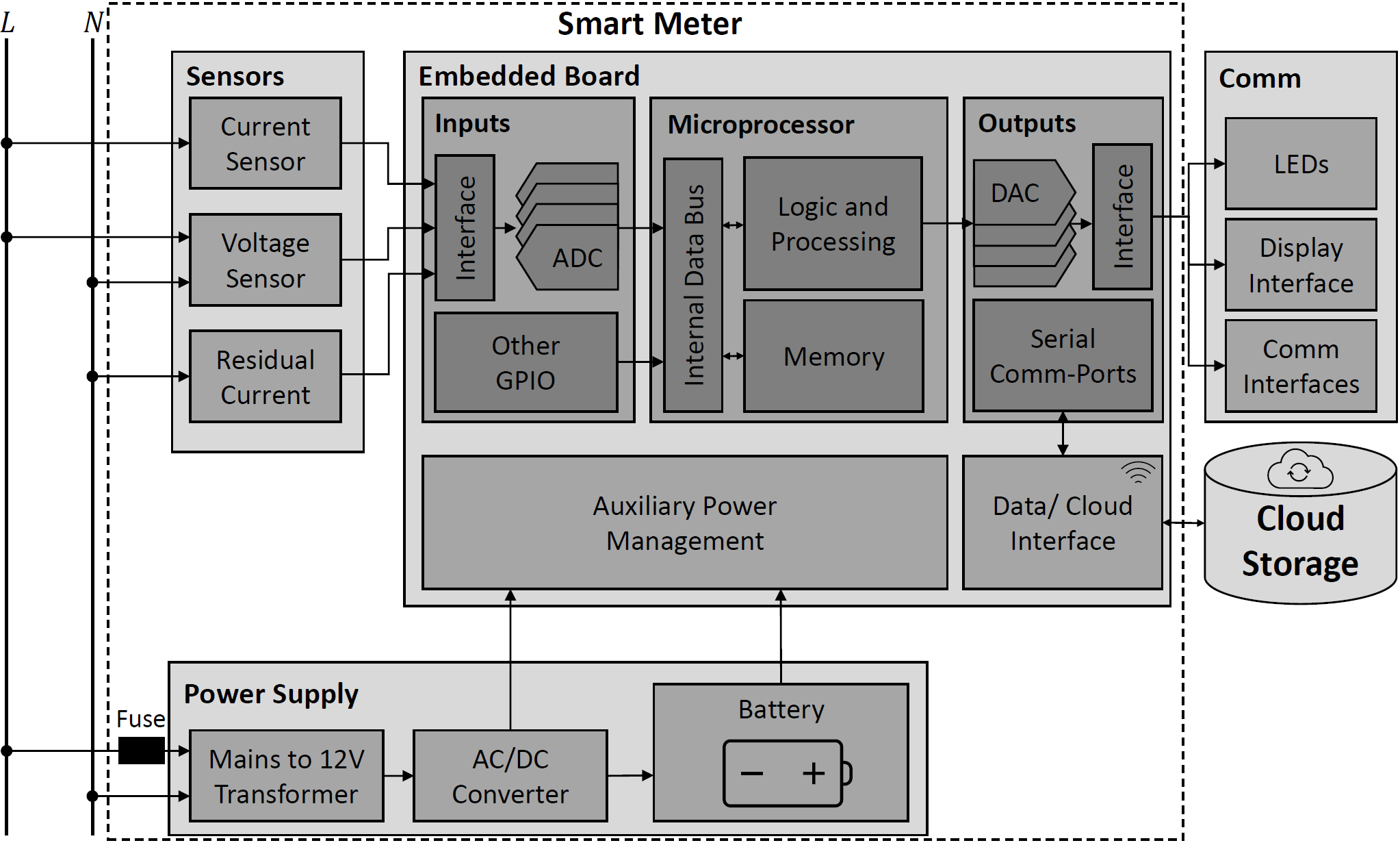Figure 3: Metering level NILM architecture.

BaseNILM is a tool for solving the energy disaggregation problem. It aims to provide a baseline systems for both new and experienced researchers within the area of energy disaggregation and Non-Intrusive Load Monitoring (NILM). For a full description please see the provided documentation under BaseNILM \docu.

Publication and Citation

The BaseNILM toolkit is part of the following NILM survey paper and tries to replicate the presented architectures and disaggregation approaches. Please cite the following paper when using the BaseNILM toolkit:

P. A. Schirmer and I. Mporas, "Non-Intrusive Load Monitoring: A Review," in IEEE Transactions on Smart Grid, vol. 14, no. 1, pp. 769-784, Jan. 2023, doi: 10.1109/TSG.2022.318959 (https://ieeexplore.ieee.org/document/9820770)

When using the high frequency operating modes please also cite the following papers depending on the approach:

P. A. Schirmer and I. Mporas, "Double Fourier Integral Analysis Based Convolutional Neural Network Regression for High-Frequency Energy Disaggregation," in IEEE Transactions on Emerging Topics in Computational Intelligence, vol. 6, no. 3, pp. 439-449, June 2022, doi: 10.1109/TETCI.2021.3086226 (https://ieeexplore.ieee.org/document/9456987)

P. A. Schirmer and I. Mporas, "2D Transformations of Energy Signals for Energy Disaggregation". Sensors 2022, 22, 7200. https://doi.org/10.3390/s2219720

Furthermore, please do also cite the corresponding publicly available datasets. As well as [1] when using the data balance option, [2] when using the WaveNet pytorch implementations and [3] when using the DSC implementation. For a complete list of all publicly available datasets please see the NILM survey paper.

Dependencies

The requirements of the BaseNILM toolkit are summarized in the requirements.txt data file. In detail, the BaseNILM toolkit was implemented using the following dependencies:

Python 3.8
Tensorflow 2.5.0
Keras 2.4.3
Scikit-Learn 1.0
Numpy
Pandas
Scipy

For GPU based calculations CUDA in combination with cuDNN has been used, utilizing the Nvidia RTX 3000 series for calculation. The following versions have been tested and proven to work with the BaseNILM toolkit:

CUDA 11.4
DNN 8.2.4
Driver 472.39

Datasets

The toolkit utilizes the following publicly available datasets, which have been pre-processed and reshaped for the users' convenience and can be found under /data.

REFIT: https://www.refitsmarthomes.org/datasets/
UKDALE: https://jack-kelly.com/data/
REDD: http://redd.csail.mit.edu/
AMPds2: https://dataverse.harvard.edu/dataset.xhtml?persistentId=doi:10.7910/DVN/FIE0S4
ECO: https://vs.inf.ethz.ch/res/show.html?what=eco-data

If the user wants to utilize their own datasets, data can be either supplied using '.xlsx', '.csv', '.mat', or '.pkl' files. Additionally, the '.h5' files converted with nilmtk can be used directly as input for the BaseNILM toolkit, but this option is not fully supported. To create a new dataset please see the attached templates. For more detailed information on possible input data file types please see the readme.txt under \data.

Limitations and Known Issues

Since the toolkit is still under development there are several things that need to be improved, are not yet implemented or lack verification. In the following a list of known issues and limitations is provided:

Loading data from nilmtk converter '.h5' files has only limited support
The focus for deep learning models is TensorFlow, while pyTorch is implemented it was not reviewed as extensively
Source Separation methods are merely implemented for completeness and are not state-of-the-art
HF data is currently only supported for '.mat' data inputs
There are minor issues for displaying and formatting units

Quick Start

For a first test run use start.py to train, test and plot a 10-fold cross validation using the AMPds2 dataset with five loads (deferrable loads). If you don't want to train simply set 'setupExp['train']==0' as the models for the example test run are already stored in BaseNILM \mdl. For changing parameters and adapting the parameters please refer to the documentation in BaseNILM \docu.

Architecture

The aim of the PyDTS toolkit is to model the input and output relation of a household energy system, namely $\hat{y}=f(X)$ where $X \in \mathbb{R}^{T \times M}$ is a feature input vector (aggregated data) of $T$ time-steps and $M$ features and $y$ is a time-series output, i.e. appliance consumption values. Mathematically the problem can be formulated as: $y(t)=\sum_{m} x_m(t) + \epsilon(t)$, where $\epsilon(t)$ is additional time dependent noise. A more generalized architecture is illustrated below:

Figure 4: Implemented generalized NILM architecture.

As can be seen, the general architecture consists of five steps namely pre-processing (e.g. resampling or filtering), window framing, feature extraction, model prediction, and post-processing (e.g. limiting the output). To better understand the theory it was also aimed to replicate this architecture in the code whenever possible

Operating Modes

The toolkit offers three different operating modes. The operating modes can be controlled using 'setupExp['sim']' option in the start.py file. The following three options are available. First, classical training and testing where a model is trained using a training and validation dataset, and tested on a testing dataset respectively. Second, hyperparameters optimization where free model parameters are optimally tuned using scikit GridSearchCV for machine learning models and keras hyperband tuner for deep learning models utilizing tensorboard. Third, general parameters can be optimized using a 2D grid search available in 'optiGrid.py'. This grid search performs exhaustive calculation for two independent parameters specified by the user.

Models

The toolkit as three different types of models implemented namely models based on Source Separation (SS), e.g. Non-Negative Matrix Factorization (NMF) or Discriminative Sparse Coding (DSC), models based on Machine/Deep Learning (ML/DL), e.g. Support Vector Machine (SVM) or Convolution Neural Networks (CNNs), and models based on Pattern Matching (PM), e.g. Dynamic Time Warping (DTW) or Minimum Variance Matching (MVM). These three model types also cover the majority of the proposed NILM approaches in the literature:

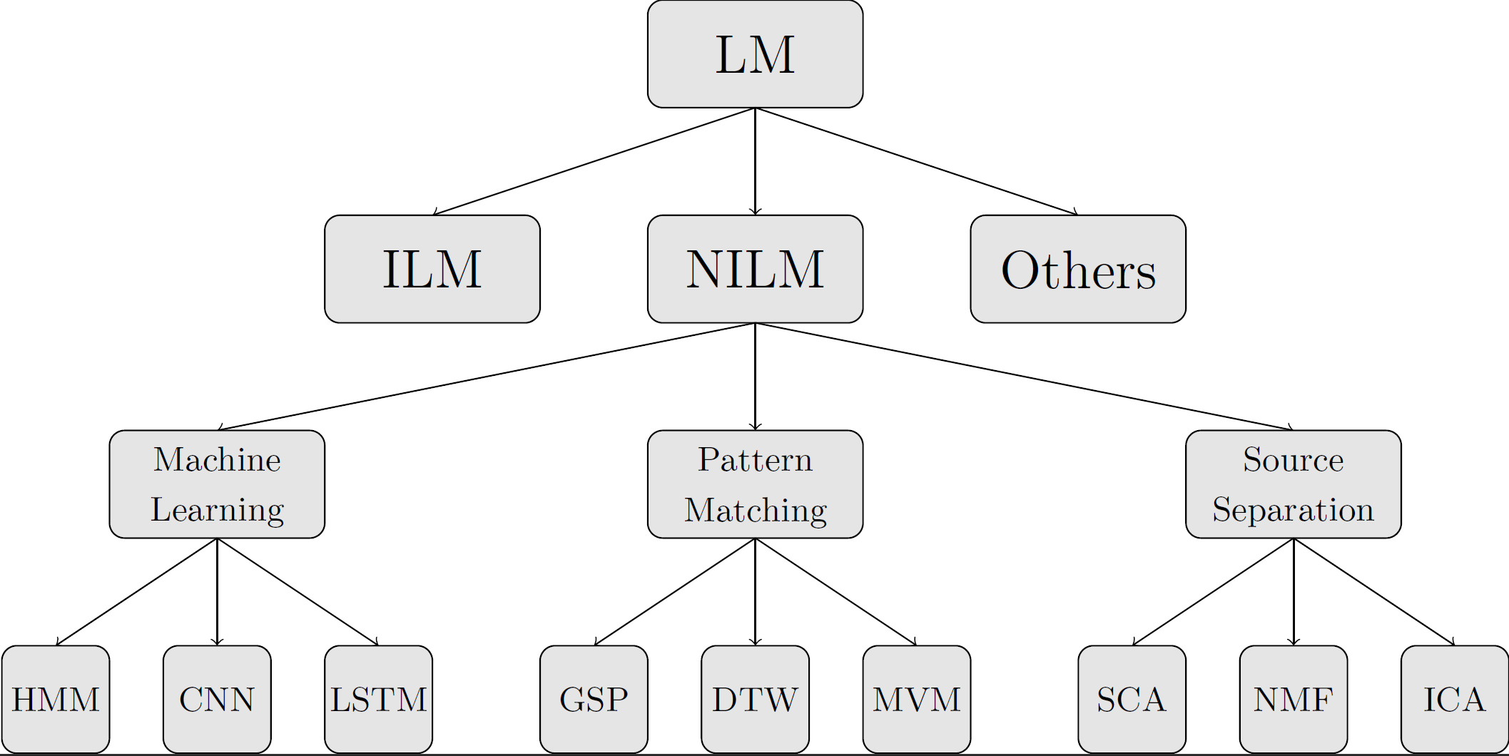Figure 5: Structure of the different NILM modeling approaches.

Exemplary Results

In the following chapter, a set of reference results is provided using the “default.txt” setup files provided in \setup. For a first test run use start.py to calculate the results presented below, which are already provided as pre-trained models under \mdl. Therefore, training is disabled in start.py. The problem considered in the default example aims to predict the power consumption of the AMPDs2 dataset (first year) using the five referable loads.

Average Results

The average results for different models and different performance metrics are provided in the table below. All results have been obtained using the default parameters of the toolkit.

Output	MAE (W)	RMSE (W)	SAE (p.u.)	TECA (%)
DNN	12.98	92.36	0.06	93.25
CNN	10.17	95.63	0.01	94.71
LSTM	14.55	97.92	0.03	92.43

As can be seen in the table above CNN outperforms all other approaches for all performance metrics.

Detailed Results

The simulation output contains four different plots. The first one provides an analysis of the input features using violin plots, a heatmap of the input and output features, as well as a feature ranking calculated by RF. The second one shows the time domain input features. The third one plots the ground truth against the predicted values and evaluates mean error and error distribution. The fourth one shows the predicted results as well as the error with respect to the ground truth for both raw values and labels.

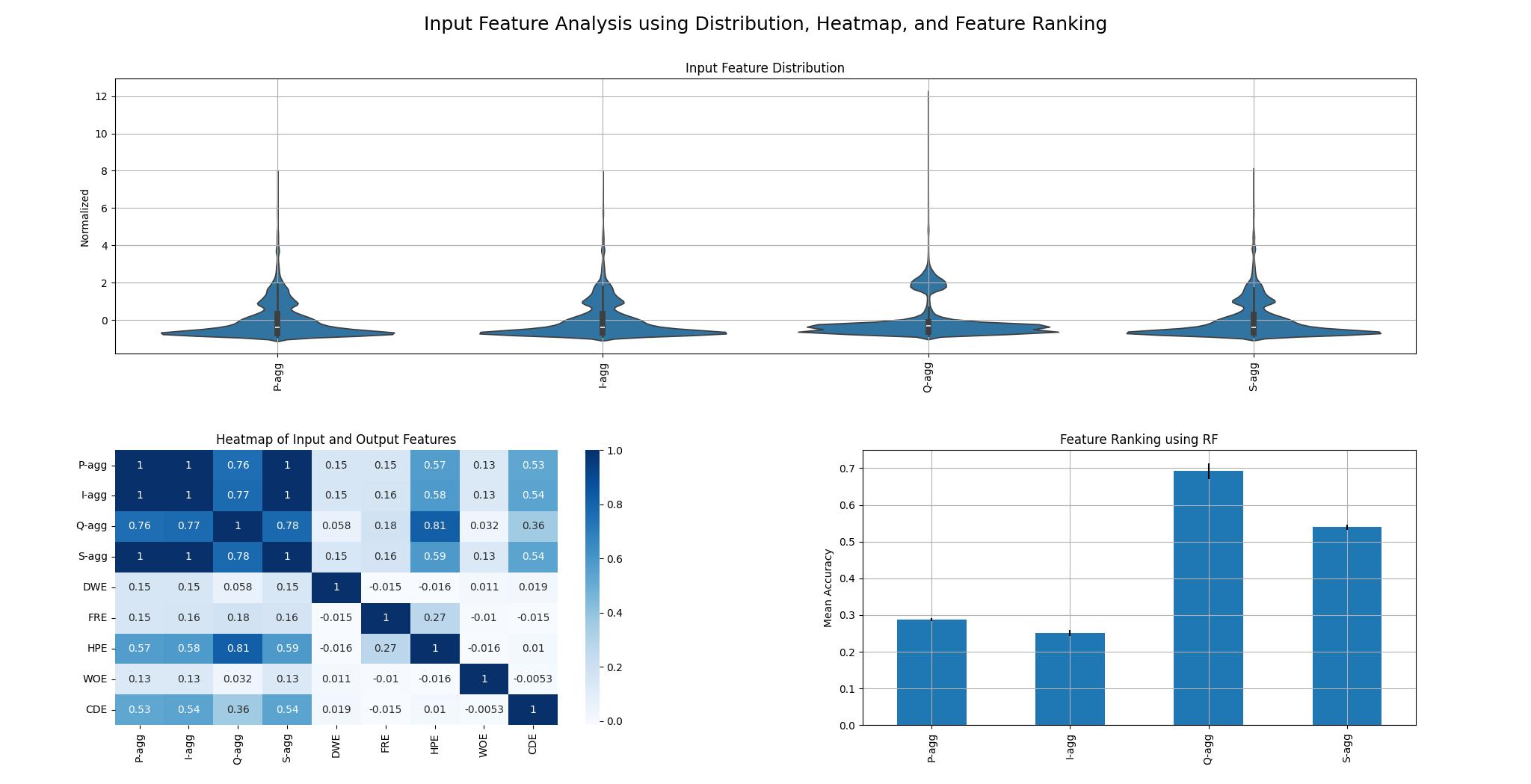Figure 6: Input feature analysis, heatmap, and feature ranking using RF classifier.

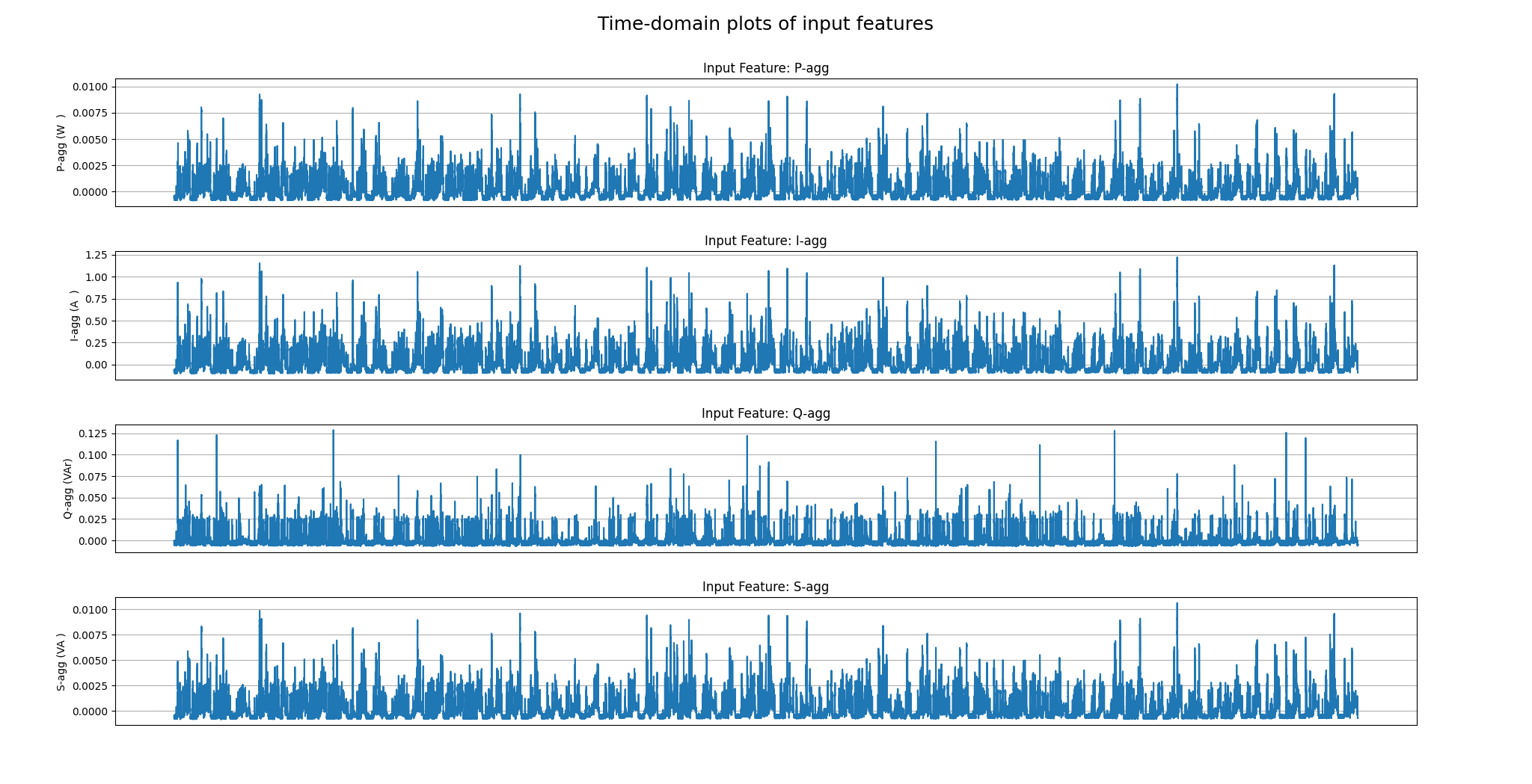Figure 7: Time-domain input features

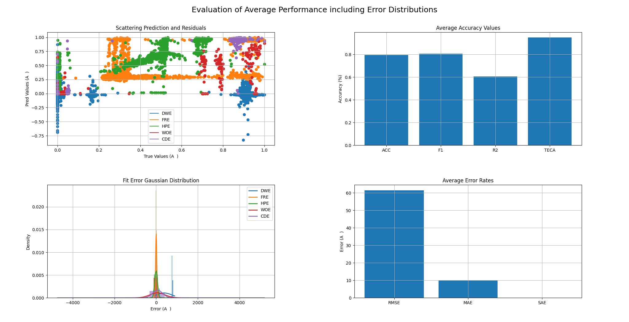Figure 8: Scattering results, Gaussian error distribution, and average accuracy values.

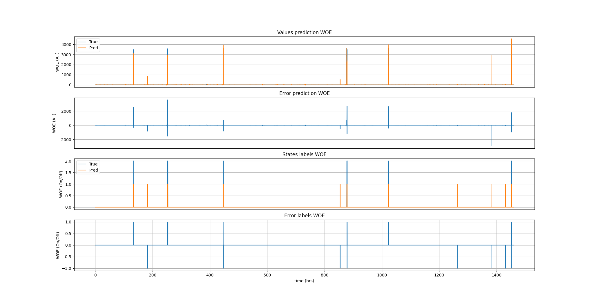Figure 9: Ground-truth and predicted values for power consumption of the WOE device.

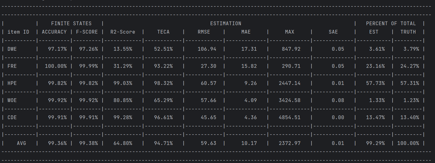
Furthermore, the console output for the best performing model (CNN) has been provided below, showing the results on device level as well as the average results.

Optimization Modes

As previously discussed the toolkit comes with two internal optimizer one performing exhaustive grid search over input variables, e.g. window length or sampling frequency, and the other one optimising hyperparameters, e.g. number of nodes and layers of a neural network, of tensorflow models. In this section, the results are presented briefly for both optimizers. The configuration can be found under \setup in the files 'defaultOptiGrid.txt' and 'defaultOptiHyper.txt'.

Window Length	Sampling Time

Figure 10: Optimal window length and sampling time based on the AMPds2 dataset.

As can be seen the optimal window length was found to be 30 minutes, while a reduction of sampling frequency goes along with a continuous reduction in disaggregation performance. Therefore, the CNN has been optimized using 30 minutes as window length as well as full sampling resolution of 1 sample/minute. The optimized CNN architecture can be found below.

Figure 11: Optimal CNN configuration based on the AMPds2 dataset.

State-of-the-Art Comparison

For comparison, we consider the AMPDs2 dataset as it is widely used and the only dataset that provides fully cleaned data, i.e. no pre-processing is necessary and thus results are exactly comparable. The results for a scenario of 10-fold cross validation using the five most used appliances in the dataset, namely ‘DWE’, 'FRE', 'HPE', ‘WOE’, and 'CDE' are presented. CNN has been used as it was found to work best for the disaggregation task. The detailed setup files can be found under \setup\compare and the numerical results are tabulated below.

Device	TECA	RMSE (W)	MAE (W)	SAE (p.u.)
DWE	61.67%	84.60	11.55	0.27
FRE	94.72%	20.80	12.31	0.03
HPE	97.31%	53.11	7.37	0.01
WOE	79.86%	70.40	3.60	0.13
CDE	97.31%	55.33	2.78	0.01
Avg	94.67%	56.85	7.52	0.00

For the comparison with the literature the same devices have been considered and different previously published methods are listed below (* note that these results are only for the first year of AMPds2 and also using current as output feature):

REF	Year	Model	TECA	RMSE (W)	MAE (W)
[4]*	2016	HMM	94.1%	-	-
[5]	2019	CNN	93.9%	-	-
[6]	2020	CNN	94.7%	-	-
[7]	2021	CNN	95.8%	-	-
BaseNILM	2023	CNN	94.7%	56.85	7.52

Development

As failure and mistakes are inextricably linked to human nature, the toolkit is obviously not perfect, thus suggestions and constructive feedback are always welcome. If you want to contribute to the BaseNILM toolkit or spotted any mistake, please contact me via: p.schirmer@herts.ac.uk

Furthermore, the following improvements are already considered for future versions:

Advanced sampling and pre-processing
Implementation of GAN models
Generation of benchmark results that can be exactly reproduced

License

The software framework is provided under the MIT license.

Version History

v.0.1: (11.07.2022) Initial version of BaseNILM
v.0.2: (19.11.2023) Complete revision of BaseNILM

Cite

References

[1] Pan, Yungang, et al. "Sequence-to-subsequence learning with conditional gan for power disaggregation." ICASSP 2020-2020 IEEE International Conference on Acoustics, Speech and Signal Processing (ICASSP). IEEE, 2020.

[2] Jiang, Jie, et al. "Deep Learning-Based Energy Disaggregation and On/Off Detection of Household Appliances." ACM Transactions on Knowledge Discovery from Data (TKDD) 15.3 (2021): 1-21.

[3] Batra, Nipun, et al. "Towards reproducible state-of-the-art energy disaggregation." Proceedings of the 6th ACM international conference on systems for energy-efficient buildings, cities, and transportation. 2019.

[4] Makonin, Stephen, et al. "Exploiting HMM sparsity to perform online real-time nonintrusive load monitoring." IEEE Transactions on smart grid 7.6 (2015): 2575-2585.

[5] Harell, Alon, Stephen Makonin, and Ivan V. Bajić. "Wavenilm: A causal neural network for power disaggregation from the complex power signal." ICASSP 2019-2019 IEEE International Conference on Acoustics, Speech and Signal Processing (ICASSP). IEEE, 2019.

[6] Schirmer, Pascal A., and Iosif Mporas. "Energy disaggregation using fractional calculus." ICASSP 2020-2020 IEEE International Conference on Acoustics, Speech and Signal Processing (ICASSP). IEEE, 2020.

[7] Schirmer, Pascal A., and Iosif Mporas. "Low-frequency energy disaggregation based on active and reactive power signatures." 2021 29th European Signal Processing Conference (EUSIPCO). IEEE, 2021.

drvshavva / BaseNILM