You can use this file as a template for your writeup if you want to submit it as a markdown file, but feel free to use some other method and submit a pdf if you prefer.
Advanced Lane Finding Project
The goals / steps of this project are the following:
- Compute the camera calibration matrix and distortion coefficients given a set of chessboard images.
- Apply a distortion correction to raw images.
- Use color transforms, gradients, etc., to create a thresholded binary image.
- Apply a perspective transform to rectify binary image ("birds-eye view").
- Detect lane pixels and fit to find the lane boundary.
- Determine the curvature of the lane and vehicle position with respect to center.
- Warp the detected lane boundaries back onto the original image.
- Output visual display of the lane boundaries and numerical estimation of lane curvature and vehicle position.
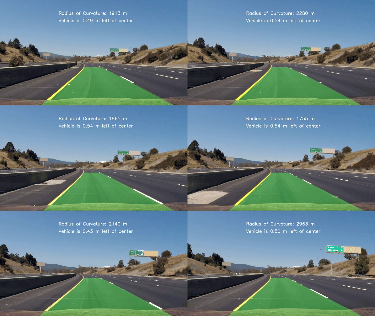
Bellow is the lane detection video output (in gif ), video can be downloaded in the root folder in the repo.
For camera calibration, first step is to compute the camera matrix and distortion coefficients. I tried following way to get the calibration parameters with CV2.
Bellow line is to get the corner points of each calibration images,
gray = cv2.cvtColor(img,cv2.COLOR_BGR2GRAY)

# Find the chessboard corners
ret, corners = cv2.findChessboardCorners(gray, (9,6),None)
Here are some samples we paint the corners, highlighted in red dots.


Then calculate the matrix and distortion coefficiencies
objpoints.append(objp)
imgpoints.append(corners)

ret, mtx, dist, rvecs, tvecs = cv2.calibrateCamera(objpoints, imgpoints, img_size,None,None)
In the return, we only need to use two parameters, mtx and dist. Others can be ignored in this project.
Following are some samples of the un-distorted images.
I start by preparing "object points", which will be the (x, y, z) coordinates of the chessboard corners in the world. Here I am assuming the chessboard is fixed on the (x, y) plane at z=0, such that the object points are the same for each calibration image. Thus, objp is just a replicated array of coordinates, and objpoints will be appended with a copy of it every time I successfully detect all chessboard corners in a test image. imgpoints will be appended with the (x, y) pixel position of each of the corners in the image plane with each successful chessboard detection.
I then used the output objpoints and imgpoints to compute the camera calibration and distortion coefficients using the cv2.calibrateCamera() function. I applied this distortion correction to the test image using the cv2.undistort() function and obtained this result:
To demonstrate this step, I will describe how I apply the distortion correction to the test images like this one:


First step is do a Gaussian Blur on the image
img = cv2.GaussianBlur(img, (kernel_size, kernel_size), 0)
Then convert to HLS color space and separate the S channel per session video
# Convert to HLS color space and separate the S channel
hls = cv2.cvtColor(img, cv2.COLOR_RGB2HLS)
s = hls[:,:,2]
Also convert to gray image
# Grayscale image
gray = cv2.cvtColor(img, cv2.COLOR_RGB2GRAY)
Finally apply the sobel function for both X and Y, and combine them together
Define sobel kernel size. Empirically use 7 as kernel size, some tuning may can get better detection results.
ksize = 7
Apply each of the thresholding functions. Here the threshold are empirical. (See last part of this write up of some discussions.)
gradx = abs_sobel_thresh(gray, orient='x', sobel_kernel=ksize, thresh=(10, 255))
grady = abs_sobel_thresh(gray, orient='y', sobel_kernel=ksize, thresh=(60, 255))
mag_binary = mag_thresh(gray, sobel_kernel=ksize, mag_thresh=(40, 255))
dir_binary = dir_threshold(gray, sobel_kernel=ksize, thresh=(.65, 1.05))
At the end, one more step which helps shorten the image process time, is to crop the image of "area of interested".
color_binary = region_of_interest(color_binary, vertices)
When process the image, we also add one step to transform the image, which is to un-distort the image based on the camera calibration parameters, matrix and distortion coefficiencies.
undist = cv2.undistort(img, mtx, dist, None, mtx)
Then use the cv2 transform the perspective
# Given src and dst points, calculate the perspective transform matrix
M = cv2.getPerspectiveTransform(src, dst)
Minv = cv2.getPerspectiveTransform(dst, src)
# Warp the image using OpenCV warpPerspective()
warped = cv2.warpPerspective(undist, M, img_size)
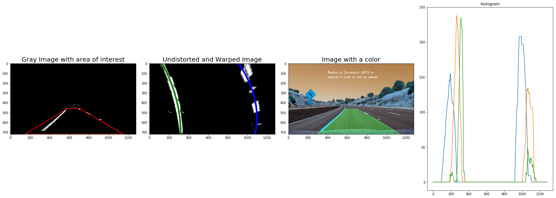
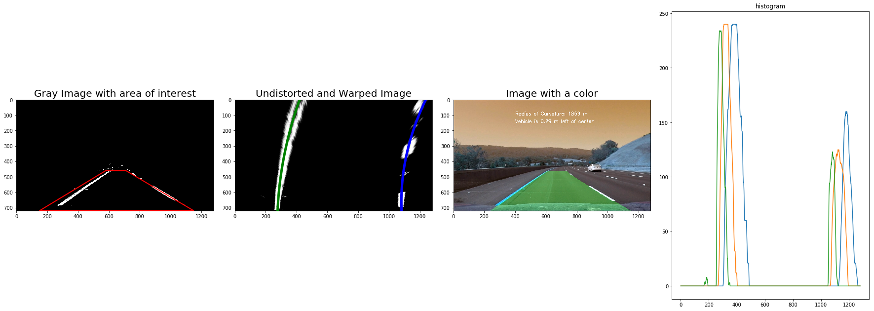
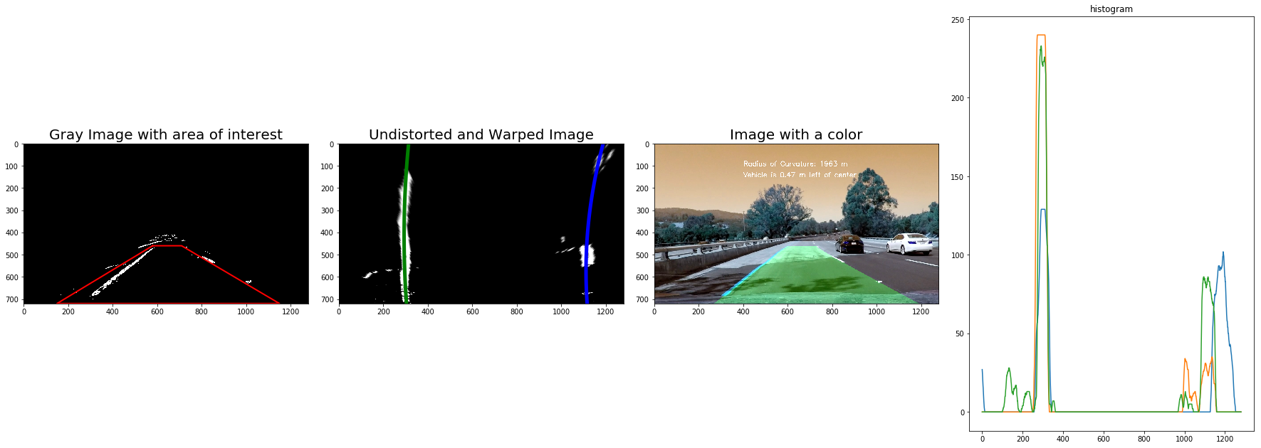
To visualize the perspective transformation clear, bellow is one sample which do the transformation on the original color image.
(In our implementation, this step done on the grey image at the end of the image pre-processing pipeline)


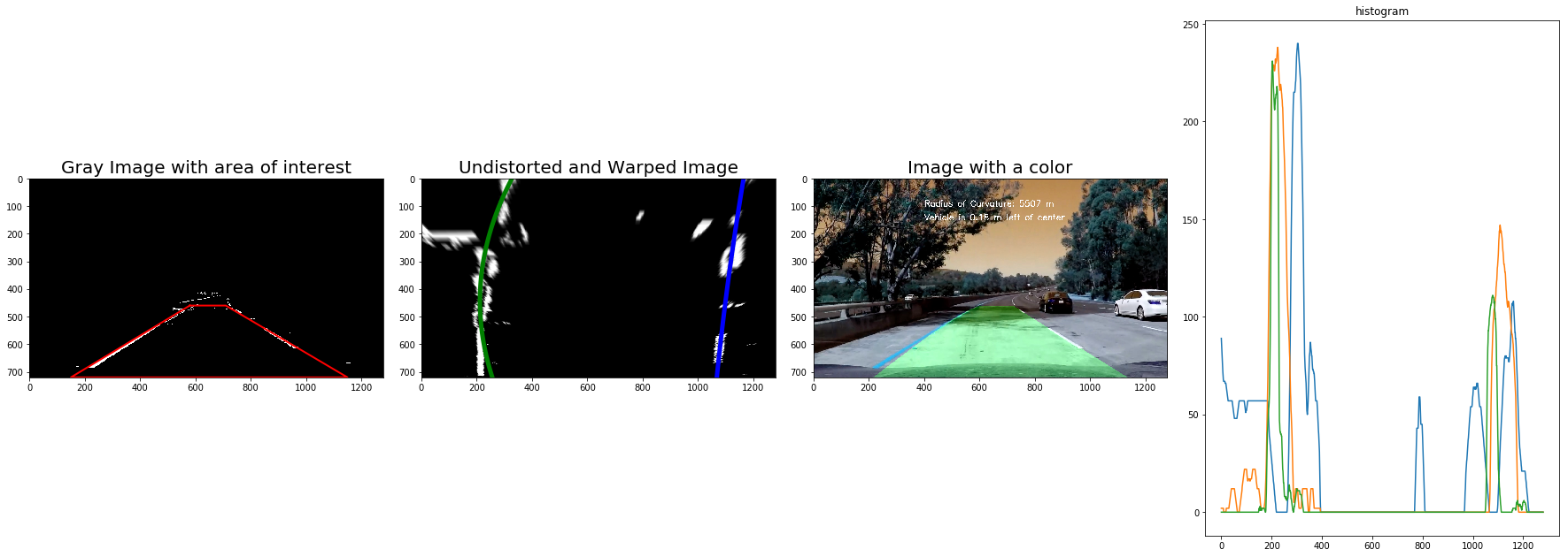
Line detection is done on the un-distorted image, which also have perspective transformed. The logic of line detection is from the course video, It will find_lanes function will detect left and right lanes from the warped image and 'n' windows will be used to identify peaks of histograms.
In this implementation, the histogram is playing a key role, the place of max value in the left side of the middle will be start point (x) of the left line, while the same for the right line.
And a moving window is used to detect the next mean of the points (above a threshold), then use polyfit function to get the parameters of the poly line.
left_fit = np.polyfit(left_lane_y, left_lane_x, 2)
At the end of the line painting, image will be transformed back to original perspective from the bird-view perspective. In the final image, we paint a green on the area between two detected lines such that the lane area is identified clearly.
Bellow is the master Function which wrapper all the Functions we discussed above, and it will be passed to the video process step.
def process_image(image):
    # Apply pipeline to the image to create black and white image
    img = pipeline(image)


    # Warp the image to make lanes parallel to each other
    top_down, perspective_M, perspective_Minv = corners_unwarp(img, mtx, dist)
    # Find the lines fitting to left and right lanes
    a, b, c, lx, ly, rx, ry, curvature = fit_lanes(top_down)
    # Return the original image with colored region
    return draw_poly(image, top_down, a, b, c, lx, ly, rx, ry, perspective_Minv, curvature)
calculated the radius of curvature of the lane and the position of the vehicle with respect to center
The way to calculate the radius basically is bery roughly, and is way more from precision, but it do help giev some estimation of the curve. Bellow is the formula used
First we define y-value where we want radius of curvature, for this I choose the maximum y-value, corresponding to the bottom of the image
y_eval = np.max(yvals)
Then since our image is pixel based, so need to do some math on the pixels. I use following algorithm to transform pixel to meter.
ym_per_pix = 30/720 # meters per pixel in y dimension
xm_per_pix = 3.7/700 # meteres per pixel in x dimension
fit_cr = np.polyfit(yvals*ym_per_pix, fitx*xm_per_pix, 2)
Finally is the formula to calculate the curvature.
curverad = ((1 + (2*fit_cr[0]*y_eval + fit_cr[1])**2)**1.5) \
                             /np.absolute(2*fit_cr[0])
When we do car position calculation, we use the image size which is pixel based. See bellow we use some hard coded pixel size to decide left or right in the lane.
position = image_shape[1]/2
left  = np.min(pts[(pts[:,1] < position) & (pts[:,0] > 700)][:,1])
right = np.max(pts[(pts[:,1] > position) & (pts[:,0] > 700)][:,1])
center = (left + right)/2
# Define conversions in x and y from pixels space to meters
xm_per_pix = 3.7/700 # meteres per pixel in x dimension
return (position - center)*xm_per_pix
Note: One thing is very important, that the calculation need to based on the original image perspective, not the bird view perspective.
I use the same way used in the P1 to process the video frame by frame, and then write to a new video mp4 file.
The final video can be found from video
- In this project, I use sobel which is different than the one used in P1, but same technologies like grey, GausioanBlur, are used in the pre-steps to pre-process images.
- There are more other ways used here than P1, like camera calibration, perspective transformation, poly line fit.
- For next step, need more time to tune the line detection algorithms, to work on the challenge videos.
- Performance wise, there should still some space which can be improved, e.g. re-use previous frame's finding, not full-scan the each frame.
- We can spend more time on the paramters tuning, like "area of interestes", "sobel kernel size", I only use HLS space and S channel, we can try some other channel with proper filter threshold may can get better results.
