#Signs of Life
##Abstract Applying reinforcement learning algorithms to real, physical, environments present a number of challenges not seen in simulated environments. In order to study and experiment with these applications, one needs a physical set up. A simple robot provides such an environment.
This article will attempt to provide the necessary instructions for anyone with a beginner level familiarity of python, to configure such a robot, and to begin to control it's movements.
Namely:
- Building the physical robot
- Powering the robot
- Initializing the robot
- Controlling the robot
- Monitoring the robot's sensors - real time and post operation.
##Building the physical robot Our simple robot will consist of 2 Dynamixel AX-12 servos (a small device whose output shaft can be positioned at various angles via it's motor), connected to the robot's body. You could get much more sophisticated by connecting several dynamixels together. There are an infinite number of configurations, but one such would create a robot similar to the following.
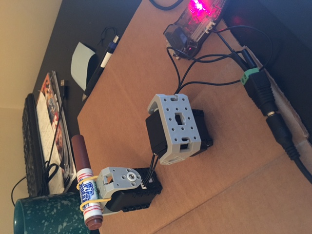
However, our setup was much simpler. As you can see, we used just two Dynamixels, each independent and with a bracket to rotate.
Brackets and frames are connected to the dynamixel to build the body. In our case, we are using nuts and bolts from the BIOLOID Nut/Bolt set http://www.robotshop.com/ca/en/robotis-bioloid-bolt-nut-set.html, and Bioloid servo brackets. With this setup, we effectively have 2 independent limbs that each have a single point of rotation (an elbow).
With this type of positioning, it's possible to instruct the dynamixel to rotate to a position which would force the bracket through it's own body. The servos obviously aren't strong enough to do so, and will shut down (a red light will be displayed) because of the increased load.
##Empowering the robot Clearly the robot will need 1) a source of power and 2) a connection to a controller (a computer).
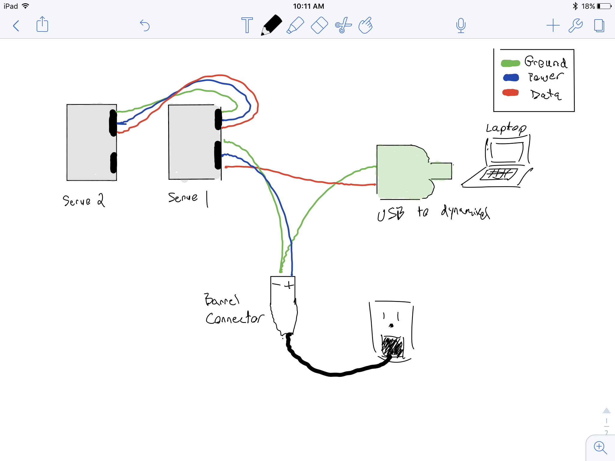
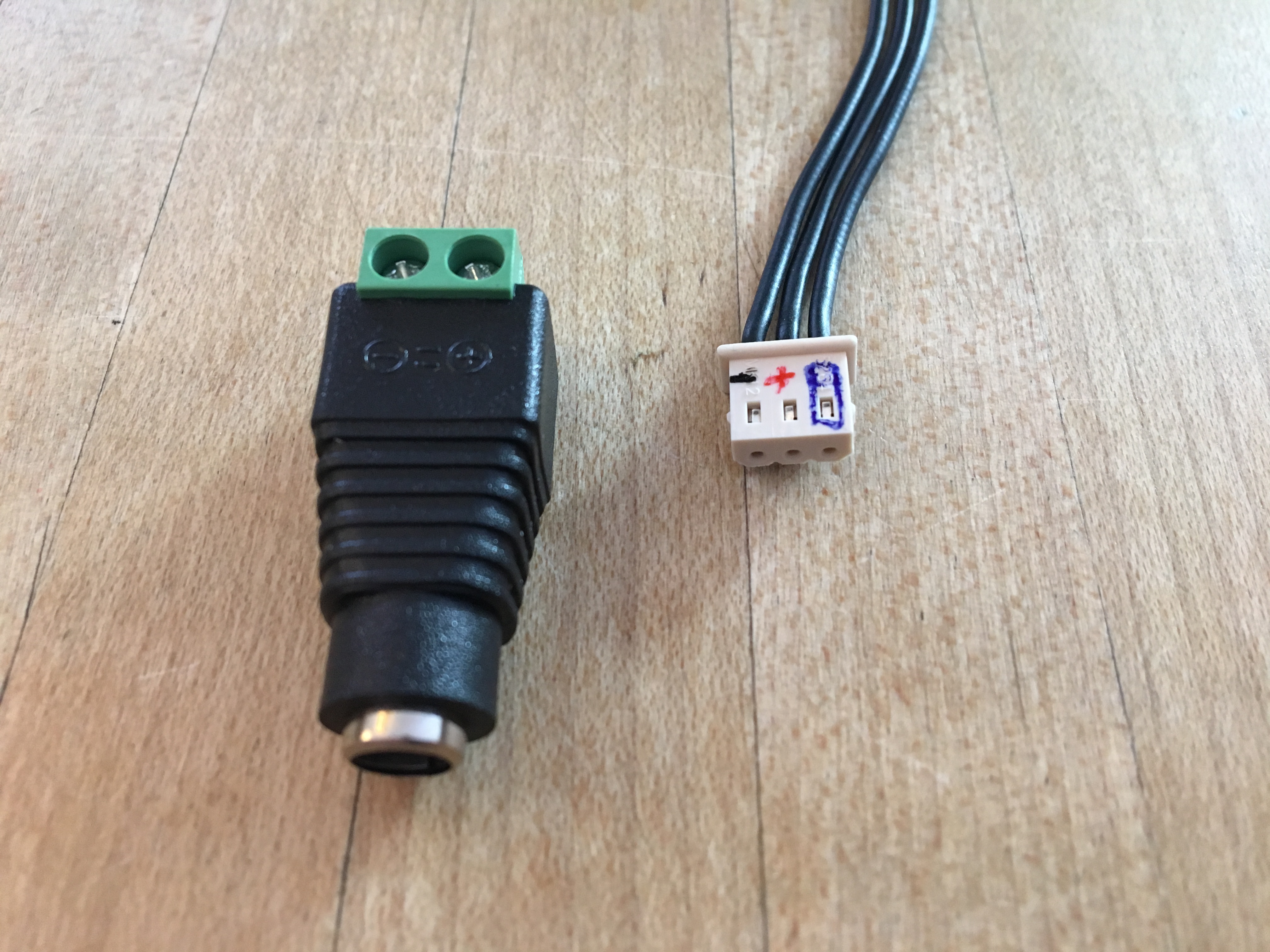
To accomplish this, a simple power harness can be fashioned using two BIOLOID 3pin cables, a power adapter, a barrel connector, a ROBOTIS USB to Dynamixel Adapter, some wire cutters, and some electrical tape. Each servo will be connected to the computer via a serial bus wire, a power source, as well as a ground wire. The ROBOTIS USB to Dynamixel needs to be connected to this data as well as ground, but does not need a power supply. The following is a simple schematic of our setup.
Using the suggested parts, the harness can be constructed using the following steps:
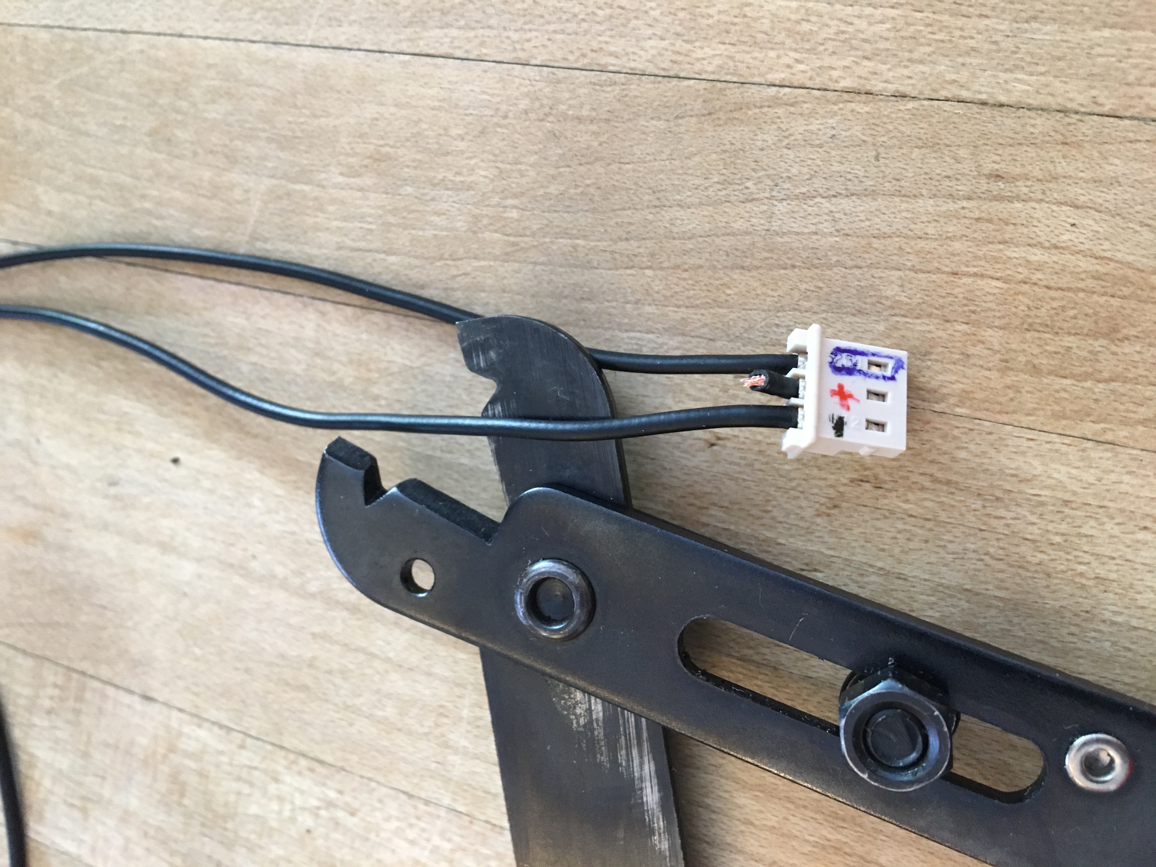
Label one of the 3pin connectors
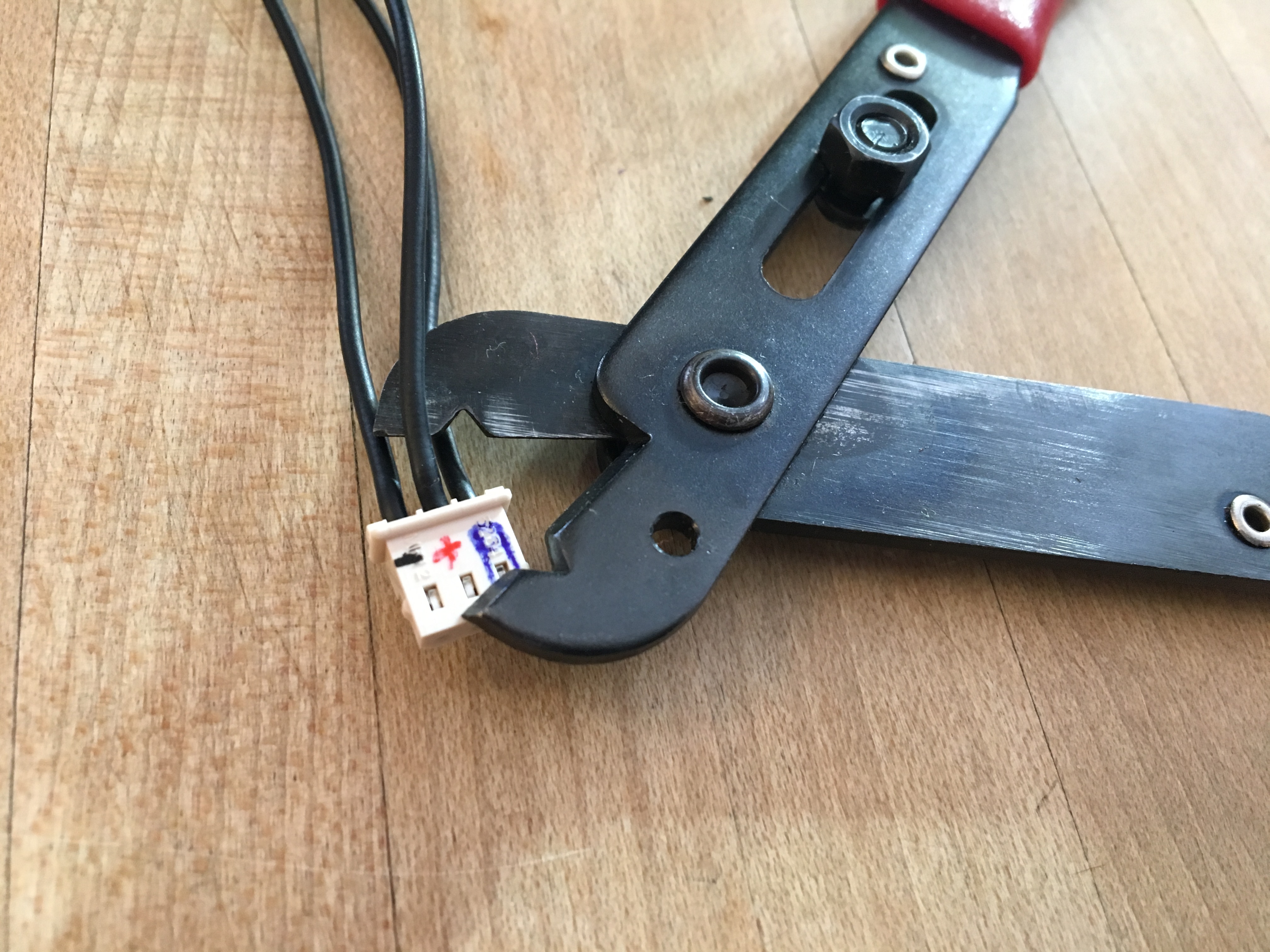
Cut positive wire supply
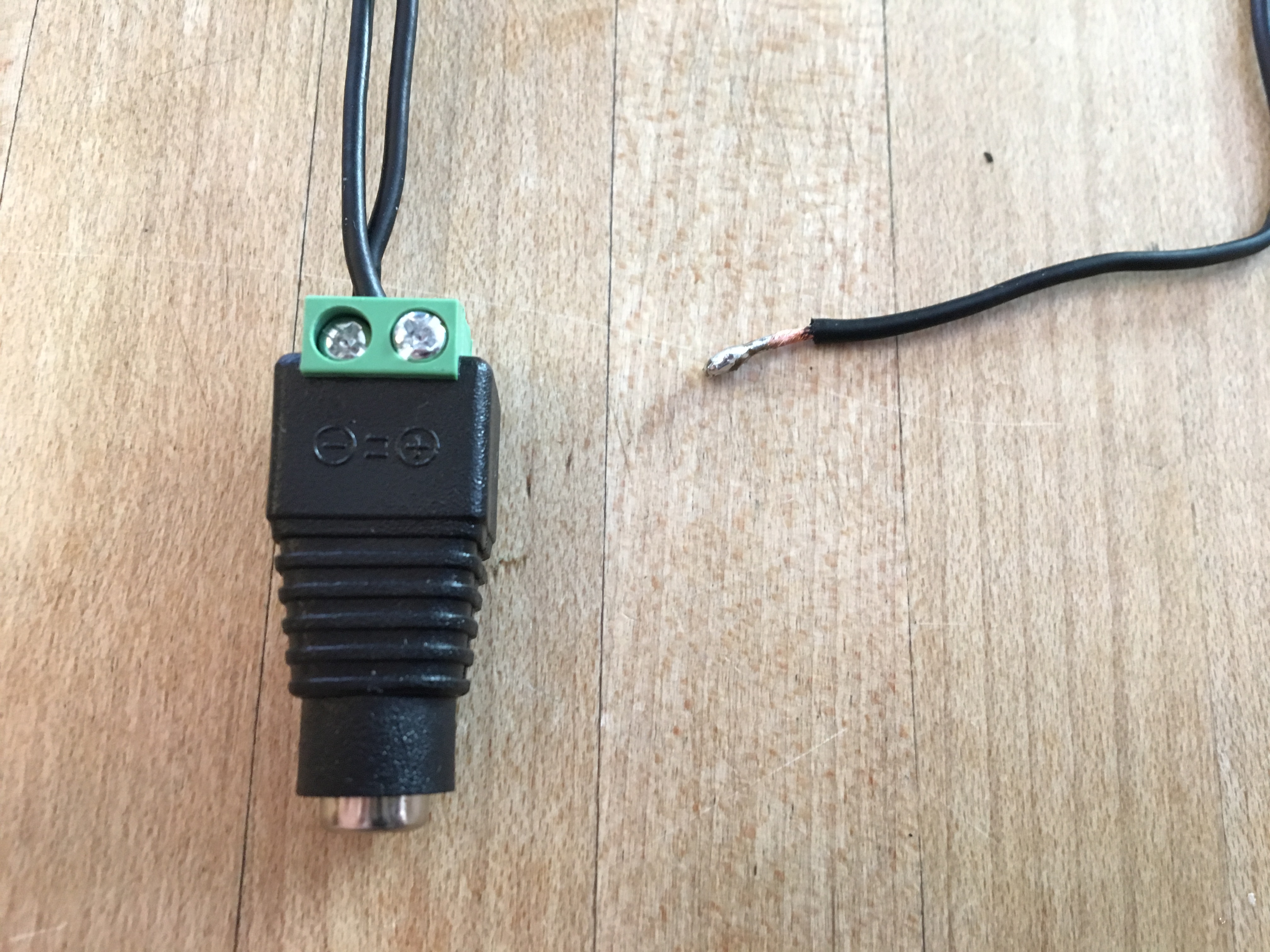
Strip the ground wire so that it can be plugged into both the power barrel and the usb to dynamixel
Fold the stripped ground wire so that it can be plugged into the barrel connector and then continue into the USB
Plug the cut and stripped positive wire to the barrel connector
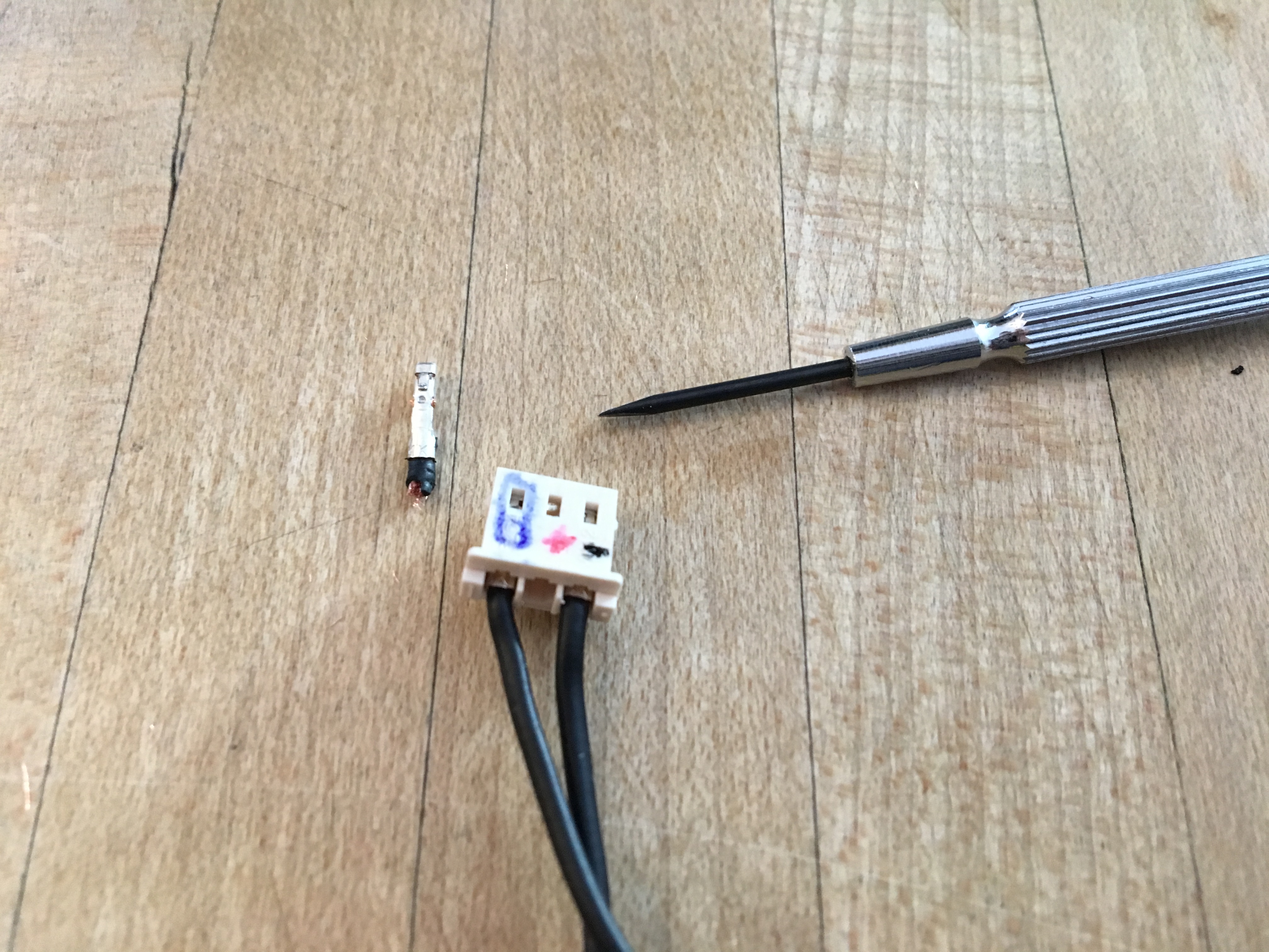
Optional - Use a screw driver to pop out the terminator wire
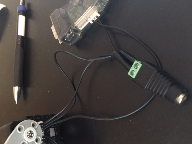
Cover any bare wire with electric tape. The final harness when plugged in will look like the following:
##Initialize the robot Once connected to the computer, the Dynamixels can configured a number of ways. Among other settings, you can restrict the allowable angles for which they can be rotated (hence preventing them from attempting to sever their own bodies). By default, the dynamixels each have an ID of 1. So it is important that we change the values to uniquely identify our servos, and prevent future collisions as future servos are added. Using lib_robotis_hack.py this can be accomplished in just a few lines of python code. The following code demonstrates connecting to the dynamixel servos and changing a basic setting.
*Note: This code doesn't exist in any of the source in this repository and should be run step by step within the python2.7 interpretor - rather than as a script:
#Note: these instructions should be run in the python interpretor one at a time rather than scripted

from lib_robotis_hack import *

# At this point, check your /dev/ directory for the location of the USB to Serial device; if in doubt, unplug the USB2Dynamixel, look at the /dev/ directory, then plug it back in and see which device has been added.

# For example, the upper right USB port on my computer gives the device: ttyUSB0

# Create the USB to Serial channel
# Use the device you identified above, and baud of 1Mbps
D = USB2Dynamixel_Device(dev_name="/dev/ttyUSB0",baudrate=1000000)

# Identify servos on the bus (should be only ONE at this point)
# Should return: "FOUND A SERVO @ ID 1"
s_list = find_servos(D)

s1.write_id(2)

# Plug in the next/remaining servo on your bus

# Rescan for servos
# Should return:
# "FOUND A SERVO @ ID 1"
# "FOUND A SERVO @ ID 2"
s_list = find_servos(D)

# Rename the second servo
# Set this servo to ID "3"
# Why, you ask? So that you can always plug in a new servo and have immediate access to it as ID "1" without overlapping with an existing servo on the bus
s2 = Robotis_Servo(D,s_list[1])
s1.write_id(3)
##Control the robot Now that the robot can be connected to and configured, we need to control how it moves. Using the lib_robotis_hack.py library, moving the robot is trivial. The following are the two function signatures used to move the servos.
class Robotis_Servo():
...

	def move_angle(self, ang, angvel=None, blocking=True):
		...

	def move_to_encoder(self, n):
move_angle will rotate the servo at the specified angular velocity until the desired angle (in radians) is achieved. By default, the call is synchronous, the call will only after the desired angle is achieved. By setting blocking=False, this call becomes async and will return before the desired angle is achieved.
move_to_encoder will rotate the servo until the desired encoding position is achieved. In the case of the dynamixels, there are 256 positions (like a clock). Each position can be achieved by calling this function.
In our case, we wanted to test the robot by randomly rotating each servo every 3 seconds. This is comparable to a learning agent learning from a random walk. To achieve this, we create a policy that returns a random angle location between 0 and 1 (we could be much more liberal with the range, but for the desired effect of twiching this is sufficient). The control thread runs and tells each servo to go to this random location every 3 seconds.
def start(self):
	#Start a loop where an action is taken every interval (time based) based on the policy

	desiredAngle = self.policy()
	try:
   	 self.servo.move_angle(desiredAngle)

	except:
    		print("!!!!!! Error moving servo")
    		pass

	threading.Timer(self.secondsAllowedPerAction, self.start).start()

def policy(self):
	#Return the angle to go to
	angle = random.uniform(0.0, 1.0)
	return angle
Here is a video of the robot performing random actions while the data is being visualized.
##Visualizing the data As the robot interacts with the world, it is important to be able to visualize the actions, and causal effect. Both in real time and after the fact.
To visualize this data in real time, we use matplot lib in interactive mode. Every 1 seconds, each servo is polled to determine it's angle, temperature, torque (load), and voltage. A plot is generated for each servo usingn the information from the last 100 seconds/inputs.
"""
#add the newest to end of arrays
self.temperatureMeasurements.append(currentTemperature)
self.torqueMeasurements.append(currentTorque)
self.angleMeasurements.append(currentAngle)
self.voltageMeasurements.append(currentVoltage)

self.torqueLine.set_ydata(self.torqueMeasurements[-self.visibleMeasurements:])
self.temperatureLine.set_ydata(self.temperatureMeasurements[-self.visibleMeasurements:])
self.angleLine.set_ydata(self.angleMeasurements[-self.visibleMeasurements:])
self.voltageLine.set_ydata(self.angleMeasurements[-self.visibleMeasurements:])

draw()
In addition to plotting the data in real time, we want to be able to recover this data. So at the same time that the data is being displayed dynamically, it is being persisted to disk in json format for later usage.
Persisting the data:
js = {'angles': self.angleMeasurements, 'torques':self.torqueMeasurements, 'temperatures':self.temperatureMeasurements, 'voltages':self.voltageMeasurements}
filename = str(self.figureIndex) + ".json"

with open(filename, 'w') as fp:
json.dump(js, fp)
Reading the data back and re-plotting:
def plotFromFile(filename):
    #Get the data from the file

    with open(filename) as jsonDataFile:
        data = json.load(jsonDataFile)

    voltages = data['voltages']
    print('Voltages: ' + str(voltages))

    temperatures = data['temperatures']
    print('Temperatures: ' + str(temperatures))

    angles = data['angles']
    print('Angles: ' + str(angles))

    torques = data['torques']
    print('Torques: ' + str(torques))

    plt.figure(1)
    plotTitle = "Servo " + str(filename)
    suptitle(plotTitle, fontsize=14, fontweight='bold')
    x = arange(0, len(temperatures), 1)
    print('x: ' + str(x))

    temperatureLine, torqueLine, angleLine, voltageLine, = plot(x, temperatures,'r', x, torques,'b', x, angles, 'g',
                                                                                    x, voltages, 'y')
    temperatureLine.axes.set_xlim(0,len(temperatures))
    temperatureLine.axes.set_ylim(-100, 100)

    temperatureLine.set_label("Temperature")
    torqueLine.set_label("Torque")
    angleLine.set_label("Angle (X 100)")
    voltageLine.set_label("Voltage")
    legend()
    grid()
    draw()
    show()
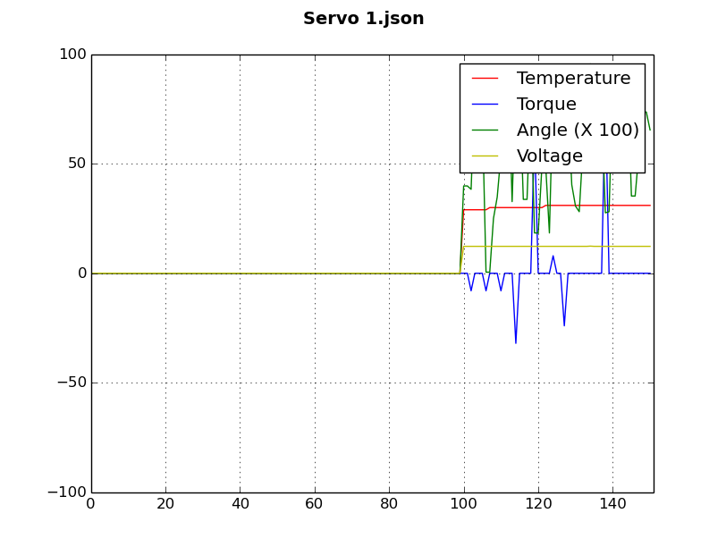
This is what the plot looks like for 1.5 minutes of activity.
##Putting it all together
To run a test where the robot will twitch indefinitely, there is a simple testRunner available in RobotController.py. This will cause the robot to twitch indefinitely until the script is killed, all the while plotting the data in real time and persisting to disk.
from RobotController import *
startTest()
