BentoBox

BentoBox is a genomic data vizualization package for R. Using grid graphics, BentoBox empowers users to programmatically and flexibly generate multi-panel figures. BentoBox accomplishes these goals by utilizing 1) a coordinate-based plotting system, and 2) edge-to-edge containerized data visualization. The coordinate-based plotting system grants users precise control over the size, position, and arrangement of plots. Its edge-to-edge plotting functions preserve the mapping between user-specified containers and the represented data. This allows users to stack plots with confidence that vertically aligned data will correspond to the same regions. For more information about BenoBox’s philosophy and design, check out the Our Philosophy page.

Specialized for genomic data, BentoBox also contains functions to read and plot multi-omic data quickly and easily. BentoBox can address an endless number of use cases, including: dynamic exploration of genomic data, arrangment into multi-omic layouts, and survey plotting for quickly viewing data across the genome. Check out our vignettes for detailed examples and suggested use cases!

Installation

BentoBox can be installed from GitHub as follows:

if (!requireNamespace("BiocManager", quietly = TRUE))
    install.packages("BiocManager")

if (!requireNamespace("remotes", quietly = TRUE))
    BiocManager::install("remotes")

remotes::install_github("PhanstielLab/BentoBox")
package.version("BentoBox")

Examples

Quick plotting

We can use any of the plotting functions to quickly plot a single data type by simply ignoring the arguments that define the plotting location (i.e. x, y, width, height, just, default.units).

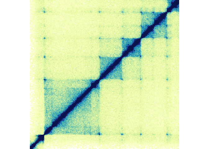
Lets demonstrate this by plotting the example Hi-C data included in bb_hicData (chr21:28000000-30300000):

## Load BentoBox
library(BentoBox)

## Load example Hi-C data
data("bb_hicData")

## Quick plot Hi-C data
hicPlot <- bb_plotHicSquare(data = bb_hicData,
                            chrom = "chr21", chromstart = 28000000, chromend = 30300000)

In addition to plotting the Hi-C Data, this creates an S3 object of class bb_hicSquare which stores all of the information about the region being plotted, the genome assembly, and any plotting parameters.

class(hicPlot)
## [1] "bb_hicSquare"

print(hicPlot)
## $chrom
## [1] "chr21"
## 
## $chromstart
## [1] 2.8e+07
## 
## $chromend
## [1] 30300000
## 
## $altchrom
## [1] "chr21"
## 
## $altchromstart
## [1] 2.8e+07
## 
## $altchromend
## [1] 30300000
## 
## $assembly
## $Genome
## [1] "hg19"
## 
## $TxDb
## [1] "TxDb.Hsapiens.UCSC.hg19.knownGene"
## 
## $OrgDb
## [1] "org.Hs.eg.db"
## 
## $gene.id.column
## [1] "ENTREZID"
## 
## $display.column
## [1] "SYMBOL"
## 
## $BSgenome
## [1] "BSgenome.Hsapiens.UCSC.hg19"
## 
## attr(,"class")
## [1] "bb_assembly"
## 
## $resolution
## [1] 10000
## 
## $x
## NULL
## 
## $y
## NULL
## 
## $width
## NULL
## 
## $height
## NULL
## 
## $just
## [1] "left" "top" 
## 
## $color_palette
## function (n) 
## {
##     x <- ramp(seq.int(0, 1, length.out = n))
##     if (ncol(x) == 4L) 
##         rgb(x[, 1L], x[, 2L], x[, 3L], x[, 4L], maxColorValue = 255)
##     else rgb(x[, 1L], x[, 2L], x[, 3L], maxColorValue = 255)
## }
## <bytecode: 0x7fb5a5932f28>
## <environment: 0x7fb5a592fdb0>
## 
## $zrange
## [1]  0 70
## 
## $half
## [1] "both"
## 
## $grobs
## gTree[GRID.gTree.1] 
## 
## attr(,"class")
## [1] "bb_hicSquare"
## attr(,"plotted")
## [1] TRUE

bb_hicSquare objects, and all objects created by bb_plot functions, can saved and used later in multi-plot arrangements (see bb_pagePlotPlace() and related vignettes). For different types of plots check out the rest of the plotting functions in the Reference section.

We can use our own data by using bb_read functions. This can be useful if there are additional processing steps required.

bb_readHic(hicFile = "path/to/file.hic", ...)

Or if no processing is required, we can simply provide the file path directly to the bb_plot function.

bb_plotHicSquare(hicData = "path/to/file.hic", ...)

Multi-plot layouts

To add annotation features to a bb_plot object, or to view multiple bb_plot objects simultaneously, we must:

Create a BentoBox coordinate page with bb_pageCreate().
Provide values for the placement arguments (x, y, width, height, just, default.units) in bb_plot functions.

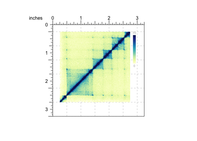
As an annotation example, lets say we want to add a color scale legend for a Hi-C plot:

## Load BentoBox
library(BentoBox)

## Load example Hi-C data
data("bb_hicData")

## Create a BentoBox page
bb_pageCreate(width = 3.25, height = 3.25, default.units = "inches")

## Plot Hi-C data with placing information
hicPlot <- bb_plotHicSquare(data = bb_hicData,
                            chrom = "chr21", chromstart = 28000000, chromend = 30300000,
                            x = 0.25, y = 0.25, width = 2.5, height = 2.5, default.units = "inches")

## Add color scale annotation
bb_annoHeatmapLegend(plot = hicPlot,
                     x = 2.85, y = 0.25, width = 0.1, height = 1.25, default.units = "inches")

By default, all placement coordinates are relative to the top right corner of the page/plot. This can be adjusted for each function individually with the just parameter. This allows us to use the most convenient coordinates to place our plot and the ability to right, left, center, top, bottom, or middle align every plotting element. For more information on plot placement, check out the vignettes.

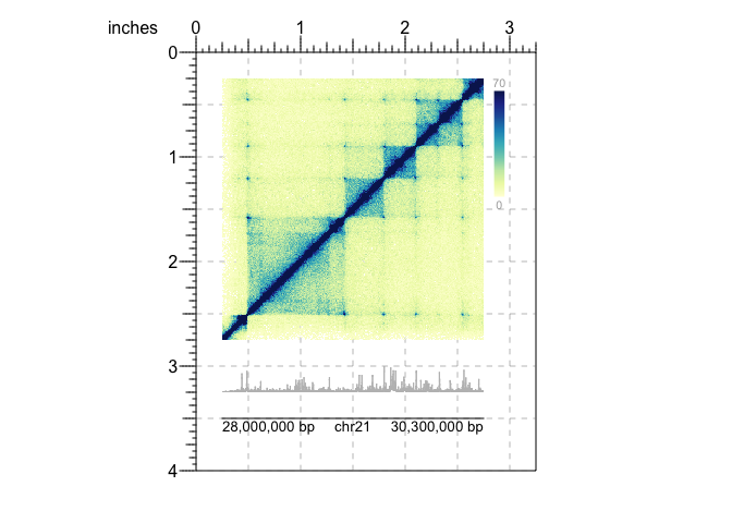
Now, let’s suppose we have both Hi-C data and signal track data such as H3K27Ac bigWig files. We could enter the region information (chr21:28000000-30300000) into both functions. But we can streamline this process by taking advantage of the bb_params() function. Since many functions share arguments, bb_params() lets us reduce repetition by defining shared arguments in one place. Furthermore, we can concatenate these bb_params objects, to create useful combinations of parameter settings. For more information about bb_params() usage, refer to the documentation or vignettes. The following code shows how we can utilize these functions to plot Hi-C data H3K27Ac signal tracks, and add a genomic label to a shared region:

## Load BentoBox
library(BentoBox)

## Load example Hi-C and signal track (H3K27Ac) data
data("bb_hicData")
data("bb_signalData")

## Define common region & plot-placement parameters
region <- bb_params(chrom = "chr21", chromstart = 28000000, chromend = 30300000)
params <- bb_params(x = 0.25, width = 2.5, default.units = "inches")

## Create a BentoBox page
bb_pageCreate(width = 3.25, height = 4, default.units = "inches")

## Plot Hi-C data with combined bb_params objects
hicPlot <- bb_plotHicSquare(data = bb_hicData,
                            params = c(region, params),
                            y = 0.25, height = params$width)

## Add color scale annotation
bb_annoHeatmapLegend(plot = hicPlot,
                     x = 2.85, y = 0.25, width = 0.1, height = 1.25, default.units = "inches")

## Plot H3K27Ac signal track
bb_plotSignal(data = bb_signalData,
              params = c(region, params),
              y = 3, height = 0.25)

## Label genome coordinates
bb_plotGenomeLabel(params = c(region, params),
                   y = 3.5, length = params$width, scale = "bp")

You might notice that using bb_params() we can remove quite a few of the plotting arguments. The only things we need to specify are the data to use and the y-coordinate to place each plot. Using c() we can also combine distinct sets of bb_params() to create different combinations of paramters for each function. We can also override arguments in bb_params() objects by defining them in local functions if needed.

Another useful feature of bb_params() is the ability to build regions and plots from gene names, given genomic annotation packages are loaded. You can check which data packages belong to which assemblies by using bb_defaultPackages(Genome) or make your own with bb_assembly():

bb_defaultPackages("hg19")
## List of 6
##  $ Genome        : chr "hg19"
##  $ TxDb          : chr "TxDb.Hsapiens.UCSC.hg19.knownGene"
##  $ OrgDb         : chr "org.Hs.eg.db"
##  $ gene.id.column: chr "ENTREZID"
##  $ display.column: chr "SYMBOL"
##  $ BSgenome      : chr "BSgenome.Hsapiens.UCSC.hg19"
##  - attr(*, "class")= chr "bb_assembly"

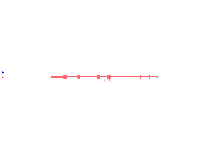
Here is an example of using bb_params() to plot the IL1B gene using the gene and geneBuffer arguments:

## Load assembly packages
library(TxDb.Hsapiens.UCSC.hg19.knownGene)
library(org.Hs.eg.db)
library(BSgenome.Hsapiens.UCSC.hg19)

## Plot IL1B with no buffer
bb_plotGenes(params = bb_params(gene = 'IL1B'))

## Plot genes with a 1000000bp (1Mb) buffer, centered on IL1B
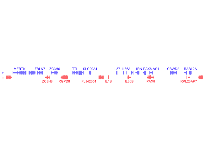
bb_plotGenes(params = bb_params(gene = 'IL1B', geneBuffer = 1000000))

A word of caution

BentoBox is incredibly flexible and functional. However, due to this flexibility and like all programming packages, it may not always prevent users from making unintentional mistakes. If plot sizes are entered incorrectly or data is mishandled, it is possible to connect multi-omic data incorrectly. Make sure you utilize package features that reduce human error and increase re-usability of code to get the most milage out of BentoBox.

dphansti / BentoBox