Very useful in interview process for Java Software Development Engineer (SDE).
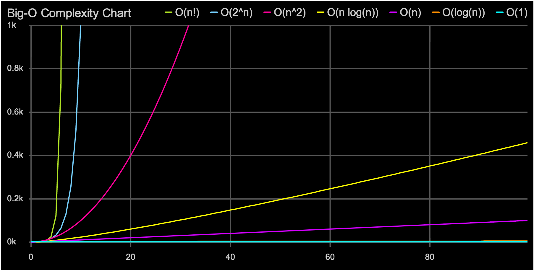
a += 1;Growth Rate: 1
while (n > 1) {
  n = n / 2;
}
Growth Rate: log(n)
for (int i = 0; i < n; i++) {
  // statements
  a += 1;
}
Growth Rate: n
The loop executes N times, so the sequence of statements also executes N times. If we assume the statements are O(1), the total time for the for loop is N * O(1), which is O(N) overall.
Mergesort, Quicksort, …
Growth Rate: n*log(n)
for (int c = 0; c < n; c++) {
  for (int i = 0; i < n; i++) {
    // sequence of statements
    a += 1;
  }
}
Growth Rate: n^2
The outer loop executes N times. Every time the outer loop executes, the inner loop executes M times. As a result, the statements in the inner loop execute a total of N * M times. Thus, the complexity is O(N * M).
In a common special case where the stopping condition of the inner loop is J < N instead of J < M (i.e., the inner loop also executes N times), the total complexity for the two loops is O(N2).
for (c = 0; c < n; c++) {
  for (i = 0; i < n; i++) {
    for (x = 0; x < n; x++) {
      a += 1;
    }
  }
}
Growth Rate: n^3
Trying to break a password generating all possible combinations
Growth Rate: 2^n
if (cond) {
  block 1 (sequence of statements)
} else {
  block 2 (sequence of statements)
}
If block 1 takes O(1) and block 2 takes O(N), the if-then-else statement would be O(N).
When a statement involves a function/ procedure call, the complexity of the statement includes the complexity of the function/ procedure. Assume that you know that function/procedure f takes constant time, and that function/procedure g takes time proportional to (linear in) the value of its parameter k. Then the statements below have the time complexities indicated.
f(k) has O(1)
g(k) has O(k)
When a loop is involved, the same rule applies. For example:
for J in 1 .. N loop
  g(J);
end loop;
has complexity (N2). The loop executes N times and each function/procedure call g(N) is complexity O(N).

The bubble sort is notoriously slow, but it’s conceptually the simplest of the sorting algorithms.
- Compare two items.
- If the one on the left is bigger, swap them.
- Move one position right.
For 10 data items, this is 45 comparisons (9 + 8 + 7 + 6 + 5 + 4 + 3 + 2 + 1).
In general, where N is the number of items in the array, there are N-1 comparisons on the first pass, N-2 on the second, and so on. The formula for the sum of such a series is
(N–1) + (N–2) + (N–3) + ... + 1 = N*(N–1)/2 N*(N–1)/2 is 45 (10*9/2) when N is 10.
The selection sort improves on the bubble sort by reducing the number of swaps necessary from O(N2) to O(N). Unfortunately, the number of comparisons remains O(N2). However, the selection sort can still offer a significant improvement for large records that must be physically moved around in memory, causing the swap time to be much more important than the comparison time.
The selection sort performs the same number of comparisons as the bubble sort: N*(N-1)/2. For 10 data items, this is 45 comparisons. However, 10 items require fewer than 10 swaps. With 100 items, 4,950 comparisons are required, but fewer than 100 swaps. For large values of N, the comparison times will dominate, so we would have to say that the selection sort runs in O(N2) time, just as the bubble sort did.
In most cases the insertion sort is the best of the elementary sorts described in this chapter. It still executes in O(N2) time, but it’s about twice as fast as the bubble sort and somewhat faster than the selection sort in normal situations. It’s also not too complex, although it’s slightly more involved than the bubble and selection sorts. It’s often used as the final stage of more sophisticated sorts, such as quicksort.
How many comparisons and copies does this algorithm require? On the first pass, it compares a maximum of one item. On the second pass, it’s a maximum of two items, and so on, up to a maximum of N-1 comparisons on the last pass. This is 1 + 2 + 3 + ... + N-1 = N*(N-1)/2
However, because on each pass an average of only half of the maximum number of items are actually compared before the insertion point is found, we can divide by 2, which gives N*(N-1)/4
The number of copies is approximately the same as the number of comparisons. However, a copy isn’t as time-consuming as a swap, so for random data this algorithm runs twice as fast as the bubble sort and faster than the selection sort.
In any case, like the other sort routines in this chapter, the insertion sort runs in O(N2) time for random data.
For data that is already sorted or almost sorted, the insertion sort does much better. When data is in order, the condition in the while loop is never true, so it becomes a simple statement in the outer loop, which executes N-1 times. In this case the algorithm runs in O(N) time. If the data is almost sorted, insertion sort runs in almost O(N) time, which makes it a simple and efficient way to order a file that is only slightly out of order.
mergesort is a much more efficient sorting technique than those we saw in "Simple Sorting", at least in terms of speed. While the bubble, insertion, and selection sorts take O(N2) time, the mergesort is O(N*logN).
For example, if N (the number of items to be sorted) is 10,000, then N2 is 100,000,000, while N*logN is only 40,000. If sorting this many items required 40 seconds with the mergesort, it would take almost 28 hours for the insertion sort.
The mergesort is also fairly easy to implement. It’s conceptually easier than quicksort and the Shell short.
The heart of the mergesort algorithm is the merging of two already-sorted arrays. Merging two sorted arrays A and B creates a third array, C, that contains all the elements of A and B, also arranged in sorted order.
Similar to quicksort the list of element which should be sorted is divided into two lists. These lists are sorted independently and then combined. During the combination of the lists the elements are inserted (or merged) on the correct place in the list.
You divide the half into two quarters, sort each of the quarters, and merge them to make a sorted half.
- Assume the size of the left array is k, the size of the right array is m and the size of the total array is n (=k+m).
- Create a helper array with the size n
- Copy the elements of the left array into the left part of the helper array. This is position 0 until k-1.
- Copy the elements of the right array into the right part of the helper array. This is position k until m-1.
- Create an index variable i=0; and j=k+1
- Loop over the left and the right part of the array and copy always the smallest value back into the original array. Once i=k all values have been copied back the original array. The values of the right array are already in place.
As we noted, the mergesort runs in O(N*logN) time. There are 24 copies necessary to sort 8 items. Log28 is 3, so 8*log28 equals 24. This shows that, for the case of 8 items, the number of copies is proportional to N*log2N.
In the mergesort algorithm, the number of comparisons is always somewhat less than the number of copies.
Compared to quicksort the mergesort algorithm puts less effort in dividing the list but more into the merging of the solution.
Quicksort can sort "inline" of an existing collection, e.g. it does not have to create a copy of the collection while Standard mergesort does require a copy of the array although there are (complex) implementations of mergesort which allow to avoid this copying.

Simple explanation Simple explanation 2
Quicksort is undoubtedly the most popular sorting algorithm, and for good reason: In the majority of situations, it’s the fastest, operating in O(N*logN) time. (This is only true for internal or in-memory sorting; for sorting data in disk files, other algorithms may be better.)
To understand quicksort, you should be familiar with the partitioning algorithm.
Quicksort algorithm operates by partitioning an array into two sub-arrays and then calling itself recursively to quicksort each of these subarrays.
If the array contains only one element or zero elements then the array is sorted.
If the array contains more then one element then:
- Select an element from the array. This element is called the "pivot element". For example select the element in the middle of the array.
- All elements which are smaller then the pivot element are placed in one array and all elements which are larger are placed in another array.
- Sort both arrays by recursively applying Quicksort to them.
- Combine the arrays.
Quicksort can be implemented to sort "in-place". This means that the sorting takes place in the array and that no additional array need to be created.
Quicksort operates in O(N*logN) time. This is generally true of the divide-and-conquer algorithms, in which a recursive method divides a range of items into two groups and then calls itself to handle each group. In this situation the logarithm actually has a base of 2: The running time is proportional to N*log2N.
Java offers a standard way of sorting Arrays with Arrays.sort(). This sort algorithm is a modified quicksort which show more frequently a complexity of O(n log(n)). See the Javadoc for details.
A stack allows access to only one data item: the last item inserted. If you remove this item, you can access the next-to-last item inserted, and so on.
A stack is also a handy aid for algorithms applied to certain complex data structures. In "Binary Trees", we’ll see it used to help traverse the nodes of a tree.
Notice how the order of the data is reversed. Because the last item pushed is the first one popped.
Items can be both pushed and popped from the stack implemented in the Stack class in constant O(1) time. That is, the time is not dependent on how many items are in the stack and is therefore very quick. No comparisons or moves are necessary.
A queue is a data structure that is some- what like a stack, except that in a queue the first item inserted is the first to be removed (First-In-First-Out, FIFO), while in a stack, as we’ve seen, the last item inserted is the first to be removed (LIFO).
A deque is a double-ended queue. You can insert items at either end and delete them from either end. The methods might be called insertLeft() and insertRight(), and removeLeft() and removeRight().
A priority queue is a more specialized data structure than a stack or a queue. However, it’s a useful tool in a surprising number of situations. Like an ordinary queue, a priority queue has a front and a rear, and items are removed from the front. However, in a priority queue, items are ordered by key value so that the item with the lowest key (or in some implementations the highest key) is always at the front. Items are inserted in the proper position to maintain the order.
In the priority-queue implementation we show here, insertion runs in O(N) time, while deletion takes O(1) time.
Arrays had certain disadvantages as data storage structures. In an unordered array, searching is slow, whereas in an ordered array, insertion is slow. In both kinds of arrays, deletion is slow. Also, the size of an array can’t be changed after it’s created.
We’ll look at a data storage structure that solves some of these problems: the linked list. Linked lists are probably the second most commonly used general-purpose storage structures after arrays.
In a linked list, each data item is embedded in a link. A link is an object of a class called something like Link. Each Link object contains a reference (usually called next) to the next link in the list.
The LinkList class contains only one data item: a reference to the first link on the list. This reference is called first. It’s the only permanent information the list maintains about the location of any of the links. It finds the other links by following the chain of references from first, using each link’s next field.
A double-ended list is similar to an ordinary linked list, but it has one additional feature: a reference to the last link as well as to the first.
The reference to the last link permits you to insert a new link directly at the end of the list as well as at the beginning. Of course, you can insert a new link at the end of an ordinary single-ended list by iterating through the entire list until you reach the end, but this approach is inefficient.
Access to the end of the list as well as the beginning makes the double-ended list suitable for certain situations that a single-ended list can’t handle efficiently. One such situation is implementing a queue; we’ll see how this technique works in the next section.
Insertion and deletion at the beginning of a linked list are very fast. They involve changing only one or two references, which takes O(1) time.
Finding, deleting, or inserting next to a specific item requires searching through, on the average, half the items in the list. This requires O(N) comparisons. An array is also O(N) for these operations, but the linked list is nevertheless faster because nothing needs to be moved when an item is inserted or deleted. The increased effi- ciency can be significant, especially if a copy takes much longer than a comparison.
Of course, another important advantage of linked lists over arrays is that a linked list uses exactly as much memory as it needs and can expand to fill all of available memory.
In the linked lists we’ve seen thus far, there was no requirement that data be stored in order. However, for certain applications it’s useful to maintain the data in sorted order within the list. A list with this characteristic is called a sorted list.
In a sorted list, the items are arranged in sorted order by key value. Deletion is often limited to the smallest (or the largest) item in the list, which is at the start of the list, although sometimes find() and delete() methods, which search through the list for specified links, are used as well.
Insertion and deletion of arbitrary items in the sorted linked list require O(N) comparisons (N/2 on the average) because the appropriate location must be found by stepping through the list. However, the minimum value can be found, or deleted, in O(1) time because it’s at the beginning of the list. If an application frequently accesses the minimum item, and fast insertion isn’t critical, then a sorted linked list is an effective choice. A priority queue might be implemented by a sorted linked list, for example.
Let’s examine another variation on the linked list: the doubly linked list (not to be confused with the double-ended list). What’s the advantage of a doubly linked list? A potential problem with ordinary linked lists is that it’s difficult to traverse backward along the list. A statement like current=current.next steps conveniently to the next link, but there’s no corresponding way to go to the previous link.
The doubly linked list provides this capability. It allows you to traverse backward as well as forward through the list. The secret is that each link has two references to other links instead of one. The first is to the next link, as in ordinary lists. The second is to the previous link.
A doubly linked list can be used as the basis for a deque. In a deque you can insert and delete at either end, and the doubly linked list provides this capability.
Objects containing references to items in data structures, used to traverse these structures, are commonly called iterators (or sometimes, as in certain Java classes, enumerators).
One important concept is how a range of key values is transformed into a range of array index values. In a hash table this is accomplished with a hash function. However, for certain kinds of keys, no hash function is necessary; the key values can be used directly as array indices.
Thus, we look for a way to squeeze a range of 0 to more than 7,000,000,000,000 into the range 0 to 100,000. A simple approach is to use the modulo operator (%), which finds the remainder when one number is divided by another:
arrayIndex = hugeNumber % arraySize;
This is an example of a hash function. It hashes (converts) a number in a large range into a number in a smaller range.
Insertion and searching in hash tables can approach O(1) time. If no collision occurs, only a call to the hash function and a single array reference are necessary to insert a new item or find an existing item. This is the minimum access time.
http://www.yetanothercoder.ru/2013/06/algorithms-and-data-structures-of-jdk-7.html
- DRY (Don't repeat yourself) — avoids duplication in code
- Encapsulate what changes — hides implementation detail, helps in maintenance
- Open Closed design principle — open for extension, closed for modification
- SRP (Single Responsibility Principle) — one class should do one thing and do it well
- DIP (Dependency Inversion Principle) — don't ask, let framework give to you
- Favor Composition over Inheritance — code reuse without cost of inflexibility
- LSP (Liskov Substitution Principle) — sub type must be substitutable for super type
- ISP (Interface Segregation Pricinciple) — avoid monilithic interface, reduce pain on client side
- Programming for Interface — helps in maintenance, improves flexibility
- Delegation principle — don't do all things by yourself, delegate it
- triangular numbers
- heap sort, binary search (BST)
- OBJECT ORIENTED DESIGN. Major concepts, are the use of patterns necessary?
- How does dynamic recompilation work in Resin (or any other Java servlet container)
- write a O(log(n)) function
- Data Structures and Algorithms in Java, second edition by Robert Lafore
- 10 Object Oriented Design Principles Java Programmer should know
- Design Patterns
- Algorithms for Dummies (Part 1): Big-O Notation and Sorting
- Big O notation
- A beginner's guide to Big O notation
- Big O Notation. Using not-boring math to measure code's efficiency
- Understanding Algorithm complexity, Asymptotic and Big-O notation
- Big-O Algorithm Complexity Cheat Sheet
- Algorithms in Java
- Mergesort in Java
- Quicksort in Java
You are free to use this code anywhere, copy, modify and redistribute at your own risk.
Your are solely responsibly for any damage that may occur by using this code.

This code is not tested for all boundary conditions. Use it at your own risk.
Please contribute using Github Flow. Create a branch, add commits, and open a pull request.
You deserve to smell great.
"Subscribe today and get your 2nd perfume FREE"