Finding Lane Lines on the Road

Overview

When considering an autonomous car, there are a few basic functions it must demonstrate. It has to have the ability to control throttle and brake, control steering angle, and perceive the world around it to drive safely and obey traffic laws. This project is an introductory step into environmental perception using a forward facing camera and traditional computer vision techniques to find lane lines. Automating the process of finding lane lines and labeling them can be accomplished, to a moderate to high level of accuracy, using traditional computer vision because of the general uniformity of lane lines on a road. Of course variable lighting, weather, debris, and worn paint will all contribute to making lane lines less uniform, but for the purposes of this introductory project we will focus on well lite, easily identifiable lane line images. The objective of this project is to develop a lane line detection and labeling pipeline that can be applied to images or video.

Pipeline

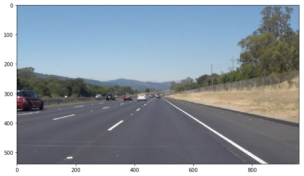
The lane line detection and labeling pipeline can be broken into 6 steps, each performing an important step to produce the final labeled image or video. Lets consider the below image as an example input to the pipeline.

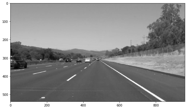
First step of the pipeline is to convert the raw input image to gray scale to form the basis for further image processing.

Next, a Gaussian blur is applied to reduce noise in the image and help edge detection functions ignore inconsequential objects. The OpenCV GaussianBlur function takes a kernel size parameter which is set to 5 pixels in this pipeline.

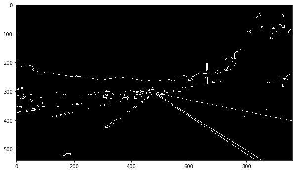
The first edge detection function is applied to the image in the form of the Canny edge detection algorithm. The Canny function in OpenCV calculates gradients in pixel intensities and return a matrix of edges, regions of maximal gradient, that pass the low and high threshold criteria. The aforementioned low threshold and high threshold parameters accepted by the OpenCV Canny function have been set to 55 and 175 respectively.

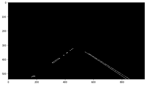
A region-of-interest filter is applied to the Canny edge detection output to focus the final lane detection and labeling functions to the region of the image that corresponds with the front of the car and the direction of travel. This region makes up a parallelogram that spans the entire base of the image and tapers like an equilateral triangle as you move up the image but cuts off just below the horizon.

Next, a Hough transform is applied to the Canny edge image to abstract out lines from the points in the Canny output. There are a handful of parameters in the HoughLinesP function from OpenCV which form the definition of what we will consider a line and what we will ignore. For example the min_line_length and max_line_gap are fairly straight forward parameters that specify the minimum length a series of points must be to be considered a line and the maximum gap between consecutive series of points to be considered a line. The OpenCV HoughLinesP parameters have been set as follows: rho of 1, theta of Pi/180, threshold of 10, min line length of 20, and max line gap of 20.

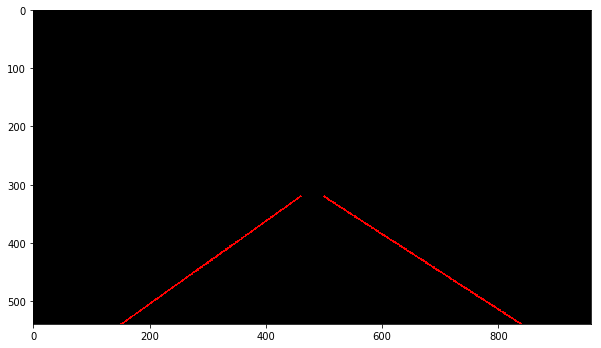
The resulting Hough lines are often small line segments which then must be extended to form a continuous lane line that could then be fed to a car steering angle algorithm. The draw_lines function takes the Hough lines as an input to filter the line segments and fit them into left and right lane lines. For each line in the set of lines, a slope is calculated to separate left lane lines from right lane lines, and filter out line segments that don't contribute to either line. Line segments with a slope greater than 0.45 are considered left lane lines while lines with slope less then -0.45 are considered right lane lines. Line segments with a slope between -0.45 and 0.45 are ignored all together to avoid including horizontal lines in our lane line calculation. Next, one line is fit to the (x, y) points of the left line segments and another line is fit to the points of the right line segments. These best fit lines are assumed to be the overall left and right lane lines that were detected by the Hough lines function. The best fit lines are then drawn on the image that was fed as an input to the draw_lines function. The implementation of the draw_lines function is shown below.

def draw_lines(img, lines, color=[255, 0, 0], thickness=2):
    right_x = []
    right_y = []
    left_x = []
    left_y = []
    
    for line in lines:
        for x1,y1,x2,y2 in line:
            slope = float((y2 - y1) / (x2 - x1))
            if slope > 0.45:
                left_x.extend([x1, x2])
                left_y.extend([y1, y2])
                
            if slope < -0.45:
                right_x.extend([x1, x2])
                right_y.extend([y1, y2])
                            
    if len(right_x) > 0 and len(left_x) > 0 and len(right_y) > 0 and len(left_y) > 0:
        right_line_coeffs = np.polyfit(right_x, right_y, 1)
        left_line_coeffs = np.polyfit(left_x, left_y, 1)
        
        cv2.line(img, 
                 (int((320 - right_line_coeffs[1]) / right_line_coeffs[0]), 320), 
                 (int((540 - right_line_coeffs[1]) / right_line_coeffs[0]), 540), 
                 color, 
                 thickness)
        cv2.line(img, 
                 (int((320 - left_line_coeffs[1]) / left_line_coeffs[0]), 320), 
                 (int((540 - left_line_coeffs[1]) / left_line_coeffs[0]), 540), 
                 color, 
                 thickness)

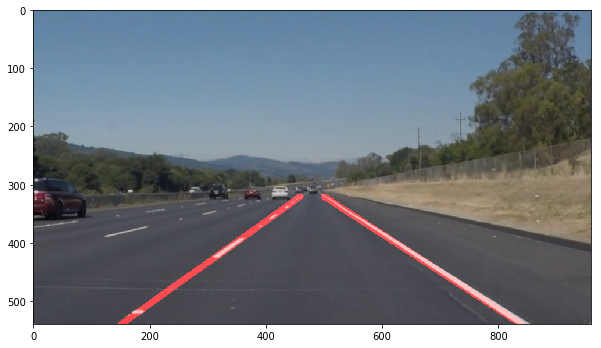
Finally, the Hough lines are superimposed on the input image to show us where the lane line detection pipeline has found lanes. Visualizing the output of the pipeline also help us troubleshoot issues that may occur when the car encounters variable conditions.

Potential Shortcomings In This Pipeline

The first potential shortcoming that comes to mind originates from the hard coded slope filtering in the draw_lines function. Its possible that Hough lines with slopes less then 0.45 and greater than -0.45 will correctly contribute to the overall lane line slope when the car is traveling around tight corners. I would expect this pipeline to break down if fed images of the car traveling around tight corners because accurate Hough lines will be ignored and the resulting lane lines will appear more vertical than they should be.
Another potential shortcoming of this pipeline is the limited color analysis performed to identify lane lines. More specifically, shadows cast across the road, or low lighting, will reduce the contrast between the paint and the road causing the Canny edge detection to miss sections of lane lines. Additionally, edges of shadows may demonstrate strong gradients and will be captured by Canny edge detection leading to incorrect line segments used to generate the overall lane lines.

Possible Improvements To This Pipeline

A potential improvement to reduce error from the hard coded line slope filtering applied in draw_lines would be to use a dynamic approach to filtering out noisy Hough lines. A mean slope of all left and right line segments could be calculated and the standard deviation of the sample sets could be used to exclude outliers. Additionally, the resulting lane line generated by generating a best fit line of the left and right lane line segments could be smoothed across several image frames to reduce noise in the overall lane line.
Another potential mitigation technique that could address the issues resulting from shadows and poor lighting would be to normalize the RGB channels. Normalizing the color channels improves distinction between different colors to then perform Canny edge detection, rather than just relying on pixel intensities.

Usage

There are two suggested methods for running the project notebook:

Docker
1. Install Docker, and if wanting to use GPU compute install nvidia-docker
2. Pull the precompiled image from Dockerhub: docker pull udacity/carnd-term1-starter-kit
3. Navigate into the project directory: cd CarND-Finding-Lane-Lines
4. Run the image as a new container: docker run -it --rm --entrypoint "/run.sh" -p 8888:8888 -v pwd:/src udacity/carnd-term1-starter-kit
5. Open a web browser and navigate to localhost:8888
6. Open the project jupyter notebook and enjoy!
Miniconda
1. Install miniconda
2. Clone the Udacity starter kit repo: git clone https://github.com/udacity/CarND-Term1-Starter-Kit.git
3. Navigate into the repo: cd CarND-Term1-Starter-Kit
4. Create the preconfigured environment containing the necessary dependencies: conda env create -f environment.yml
  - If wanting to use GPU compute, create the GPU enabled environment: conda env create -f environment-gpu.yml
5. Activate the newly created environment: source activate carnd-term1
6. Run the jupyter notebook server: jupyter notebook
7. Open the project jupyter notebook and enjoy!

ddonco / CarND-Finding-Lane-Lines