davidjesusacu / geometry-processing-registration

Registration assignment for Geometry Processing course

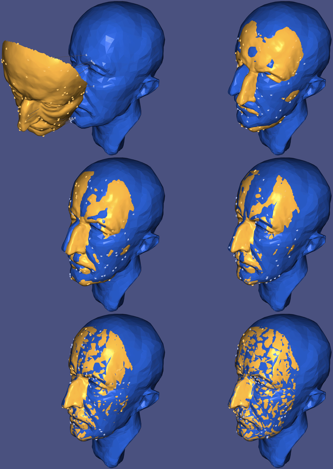
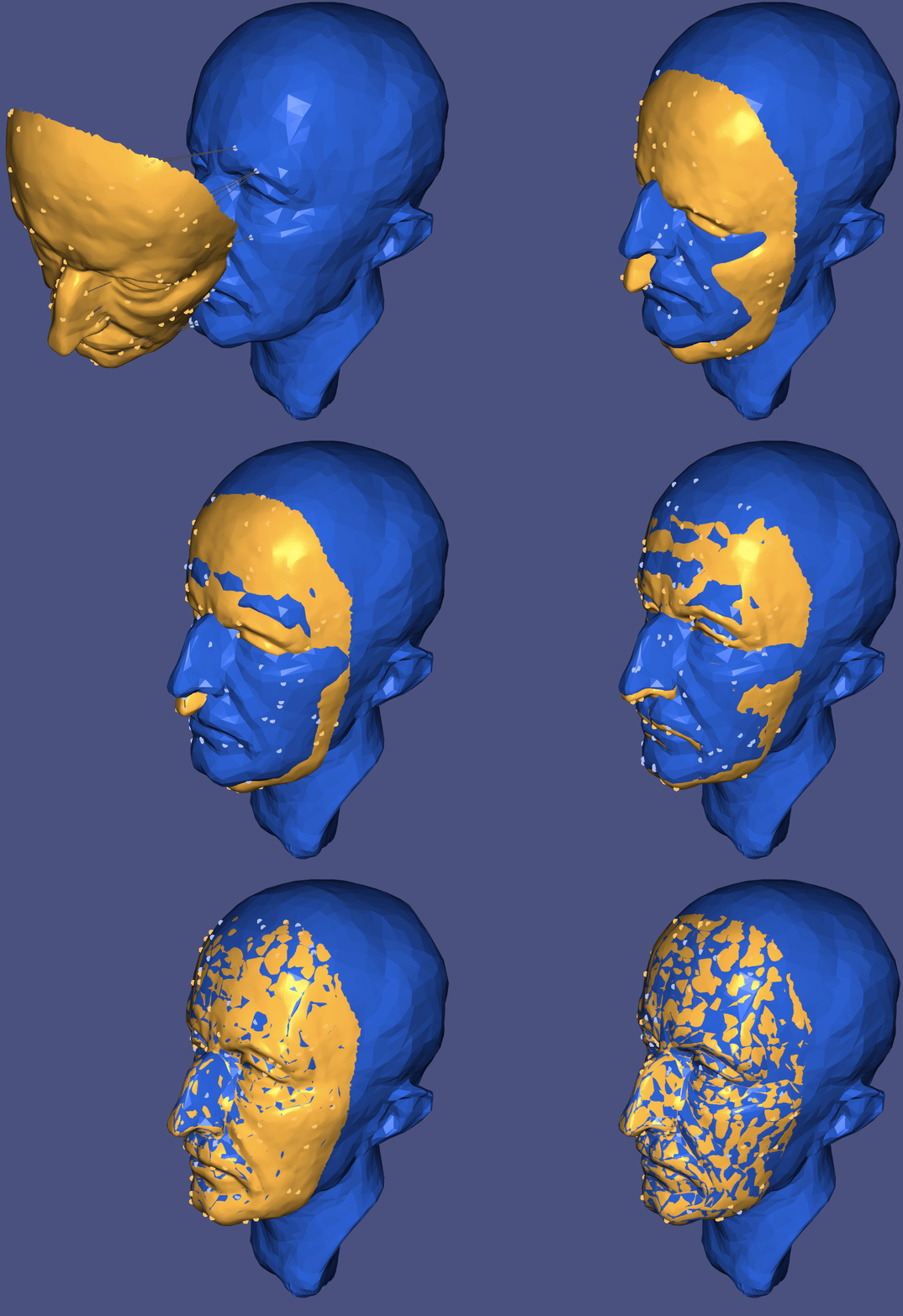
Geometry Processing – Registration

To get started: Fork this repository then issue

git clone --recursive http://github.com/[username]/geometry-processing-registration.git

Installation, Layout, and Compilation

See introduction.

Execution

Once built, you can execute the assignment from inside the build/ using

./registration [path to mesh1.obj] [path to mesh2.obj]

Background

In this assignment, we will be implementing a version of the iterative closest point (ICP), not to be confused with Insane Clown Posse.

Rather than registering multiple point clouds, we will register multiple triangle mesh surfaces.

This algorithm and its many variants has been use for quite some time to align discrete shapes. One of the first descriptions is given in "A Method for Registration of 3-D Shapes" by Besl & McKay 1992. However, the award-winning PhD thesis of Sofien Bouaziz ("Realtime Face Tracking and Animation" 2015, section 3.2-3.3) contains a more modern view that unifies many of the variants with respect to how they impact the same core optimization problem.

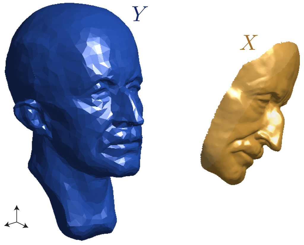
For our assignment, we will assume that we have a triangle mesh representing a complete scan of the surface $Y$ of some rigid object and a new partial scan of that surface $X$.

These meshes will not have the same number of vertices or the even the same topology. We will first explore different ways to measure how well aligned two surfaces are and then how to optimize the rigid alignment of the partial surface $X$ to the complete surface $Y$.

Hausdorff distance

We would like to compute a single scalar number that measures how poorly two surfaces are matched. In other words, we would like to measure the distance between two surfaces. Let's start by reviewing more familiar distances:

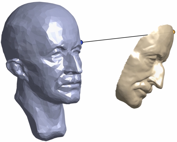
Point-to-point distance

The usually Euclidean distance between two points $\x$ and $\y$ is the $L²$ norm of their difference :

\[ d(\x,\y) = ‖\x - \y‖. \]

Point-to-projection distance

When we consider the distance between a point $\x$ and some larger object $Y$ (a line, a circle, a surface), the natural extension is to take the distance to the closest point $\y$ on $Y$:

\[ d(\x,Y) = \inf_{\y ∈ Y} d(\x,\y). \]

written in this way the infimum considers all possible points $\y$ and keeps the minimum distance. We may equivalently write this distance instead as simply the point-to-point distance between $\x$ and the closest-point projection $P_Y(\x)$:

\[ d(\x,Y) = d((\x,P_Y(\x)) = ‖\x - P_Y(\x)‖. \]

If $Y$ is a smooth surface, this projection will also be an orthogonal projection.

Directed Hausdorff distance

We might be tempted to define the distance from surface $X$ to $Y$ as the infimum of point-to-projection distances over all points $\x$ on $X$:

\[ D_\text{inf}(X,Y) = \inf_{\x ∈ X} ‖\x - P_Y(\x)‖, \]

but this will not be useful for registering two surfaces: it will measure zero if even just a single point of $\x$ happens to lie on $Y$. Imagine the noses of two faces touching at their tips.

Instead, we should take the supremum of point-to-projection distances over all points $\x$ on $X$:

\[ D_{\overrightarrow{H}}(X,Y) = \sup_{\x ∈ X} ‖\x - P_Y(\x)‖. \]

This surface-to-surface distance measure is called the directed Hausdorff distance. We may interpret this as taking the worst of the best: we let each point $\x$ on $X$ declare its shortest distance to $Y$ and then keep the longest of those.

It is easy to verify that $D_{\overrightarrow{H}}$ will only equal zero if all points on $X$ also lie exactly on $Y$.

The converse is not true: if $D_{\overrightarrow{H}}=0$ there may still be points on $Y$ that do not lie on $X$. In other words, in general the directed Hausdorff distance from surface $X$ to surface $Y$ will not equal the Hausdorff distance from surface $Y$ to surface $X$:

\[ D_{\overrightarrow{H}}(X,Y) ≠ D_{\overrightarrow{H}}(Y,X). \]

directed Hausdorff distance between triangle meshes

We can approximate a lower bound on the Hausdorff distance between two meshes by densely sampling surfaces $X$ and $Y$. We will discuss sampling methods, later. For now consider that we have chosen a set $\P_X$ of $k$ points on $X$ (each point might lie at a vertex, along an edge, or inside a triangle). The directed Hausdorff distance from $X$ to another triangle mesh $Y$ must be greater than the directed Hausdorff distance from this point cloud $\P_X$ to $Y$:

\[ D_{\overrightarrow{H}}(X,Y) ≥ D_{\overrightarrow{H}}(\P_X,Y) = \max_{i=1}^k ‖\p_i - P_Y(\p_i)‖, \]

where we should be careful to ensure that the projection $P_Y(\p_i)$ of the point $\p_i$ onto the triangle mesh $Y$ might lie at a vertex, along an edge or inside a triangle.

As our sampling $\P_X$ becomes denser and denser on $X$ this lower bound will approach the true directed Hausdorff distance. Unfortunately, an efficient upper bound is significantly more difficult to design.

Hausdorff distance for alignment optimization

Even if it were cheap to compute, Hausdorff distance is difficult to optimize when aligning two surfaces. If we treat the Hausdorff distance between surfaces $X$ and $Y$ as an energy to be minimized, then only change to the surfaces that will decrease the energy will be moving the (in general) isolated point on $X$ and isolated point on $Y$ generating the maximum-minimum distance. In effect, the rest of the surface does not even matter or effect the Hausdorff distance. This, or any type of $L^∞$ norm, will be much more difficult to optimize.

Hausdorff distance can serve as a validation measure, while we turn to $L²$ norms for optimization.

Integrated closest-point distance

We would like a distance measure between two surfaces that---like Hausdorff distance---does not require a shared parameterization. Unlike Hausdorff distance, we would like this distance to diffuse the measurement over the entire surfaces rather than generate it from the sole worst offender. We can accomplish this by replacing the supremum in the Hausdorff distance ($L^∞$) with a integral of squared distances ($L²$). Let us first define a directed closest-point distance from a surface $X$ to another surface $Y$, as the integral of the squared distance from every point $\x$ on $X$ to its closest-point projection $P_Y(\x)$ on the surfaces $Y$:

\[ D_{\overrightarrow{C}}(X,Y) = \sqrt{\ ∫\limits_{\x∈X} ‖\x - P_Y(\x) ‖² ;dA }. \]

This distance will only be zero if all points on $X$ also lie on $Y$, but when it is non-zero it is summing/averaging/diffusing the distance measures of all of the points.

This distance is suitable to define a matching energy, but is not necessarily welcoming for optimization: the function inside the square is non-linear. Let's dig into it a bit. We'll define a directed matching energy $E_{\overrightarrow{C}}(Z,Y)$ from $Z$ to $Y$ to be the squared directed closest point distance from $X$ to $Y$:

\[ E_{\overrightarrow{C}}(Z,Y) = ∫\limits_{\z∈Z} ‖\z - P_Y(\z) ‖² ;dA = ∫\limits_{\z∈Z} ‖f_Y(\z) ‖² ;dA \]

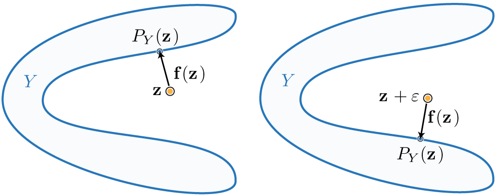
where we introduce the proximity function $\f_Y:\R³→\R³$ defined simply as the vector from a point $\z$ to its closest-point projection onto $Y$:

\[ \f(\z) = \z - P_Y(\z). \]

Suppose $Y$ was not a surface, but just a single point $Y = {\y}$. In this case, $\f(\z) = \z - \y$ is clearly linear in $\z$.

Similarly, suppose $Y$ was an infinite plane $Y = {\y | (\y-\p)⋅\n = 0}$ defined by some point $\p$ on the plane and the plane's unit normal vector $\n$. Then $\f(\z) = ((\z-\p)⋅\n)\n)$ is also linear in $\z$.

But in general, if $Y$ is an interesting surface $\f(\z)$ will be non-linear; it might not even be a continuous function.

In optimization, a common successful strategy to minimize energies composed of squaring a non-linear functions $\f$ is to linearize the function about a current input value (i.e., a current guess $\z₀$), minimize the energy built from this linearization, then re-linearize around that solution, and then repeat.

This is the core idea behind gradient descent and the Gauss-Newton methods:

minimize f(z)²
  z₀ ← initial guess
  repeat until convergence
    f₀ ← linearize f(z) around z₀
    z₀ ← minimize f₀(z)²

Since our $\f$ is a geometric function, we can derive its linearizations geometrically.

Constant function approximation

If we make the convenient---however unrealistic---assumption that in the neighborhood of the closest-point projection $P_Y(\z₀)$ of the current guess $\z₀$ the surface $Y$ is simply the point $P_Y(\z₀)$ (perhaps imagine that $Y$ is makes a sharp needle-like point at $P_Y(\z₀)$ or that $Y$ is very far away from $\x$), then we can approximate $\f(\z)$ in the proximity of our current guess $\z₀$ as the vector between the input point $\z$ and $P_Y(\z₀)$:

\[ \f(\z) \approx \f_\text{point}(\z) = \z-P_Y(\z₀) \]

In effect, we are assuming that the surface $Y$ is constant function of its parameterization: $\y(u,v) = P_Y(\z₀)$.

Minimizing $E_{\overrightarrow{C}}$ iteratively using this linearization (or rather constantization) of $\f$ is equivalent to the gradient descent. We have simply derived our gradients geometrically.

Linear function approximation

If we make make a slightly more appropriate assumption that in the neighborhood of the $P_Y(\z₀)$ the surface $Y$ is a plane, then we can improve this approximation while keeping $\f$ linear in $\z$:

\[ \f(\z) \approx \f_\text{plane}(\z) = ((\z-P_Y(\z₀))⋅\n) \n. \]

where the plane that best approximates $Y$ locally near $P_Y(\z₀)$ is the tangent plane defined by the normal vector $\n$ at $P_Y(\z₀)$.

Minimizing $E_{\overrightarrow{C}}$ iteratively using this linearization of $\f$ is equivalent to the Gauss-Newton method. We have simply derived our linear approximation geometrically.

Equipped with these linearizations, we may now describe an optimization algorithm for minimizing the matching energy between a surface $Z$ and another surface $Y$.

Iterative closest point algorithm

So far we have derived distances between a surface $Z$ and another surface $Y$. In our rigid alignment and registration problem, we would like to transform one surface $X$ into a new surface $T(X) = Z$ so that it best aligns with/matches the other surface $Y$. Further we require that $T$ is a rigid transformation: $T(\x) = \Rot \x + \t$ for some rotation matrix $\Rot ∈ SO(3) ⊂ \R^{3×3}$ (i.e., an orthogonal matrix with determinant 1) and translation vector $\t∈\R³$.

Our matching problem can be written as an optimization problem to find the best possible rotation $\Rot$ and translation $\t$ that match surface $X$ to surface $Y$:

\[ \mathop{\text{minimize}}{\t∈\R³,\ \Rot ∈ SO(3)} ∫\limits{\x∈X} ‖\Rot \x + \t - P_Y(T(\x)) ‖² ;dA \]

Even if $X$ is a triangle mesh, it is difficult to integrate over all points on the surface of $X$. At any point, we can approximate this energy by summing over a point-sampling of $X$:

\[ \mathop{\text{minimize}}{\t∈\R³,\ \Rot ∈ SO(3)} ∑{i=1}^k ‖\Rot \x_i + \t - P_Y(T(\x_i)) ‖², \]

where $\X ∈ \R^{k×3}$ is a set of $k$ points on $X$ so that each point $\x_i$ might lie at a vertex, along an edge, or inside a triangle. We defer discussion of how to sample a triangle mesh surface.

Pseudocode

As the name implies, the method proceeds by iteratively finding the closest point on $Y$ to the current rigid transformation $\Rot \x + \t$ of each sample point $\x$ in $\X$ and then minimizing the linearized energy to update the rotation $\Rot$ and translation $\t$.

If $V_X$ and $F_X$ are the vertices and faces of a triangle mesh surface $X$ (and correspondingly for $Y$), then we can summarize a generic ICP algorithm in pseudocode:

icp V_X, F_X, V_Y, F_Y
  R,t ← initialize (e.g., set to identity transformation)
  repeat until convergence
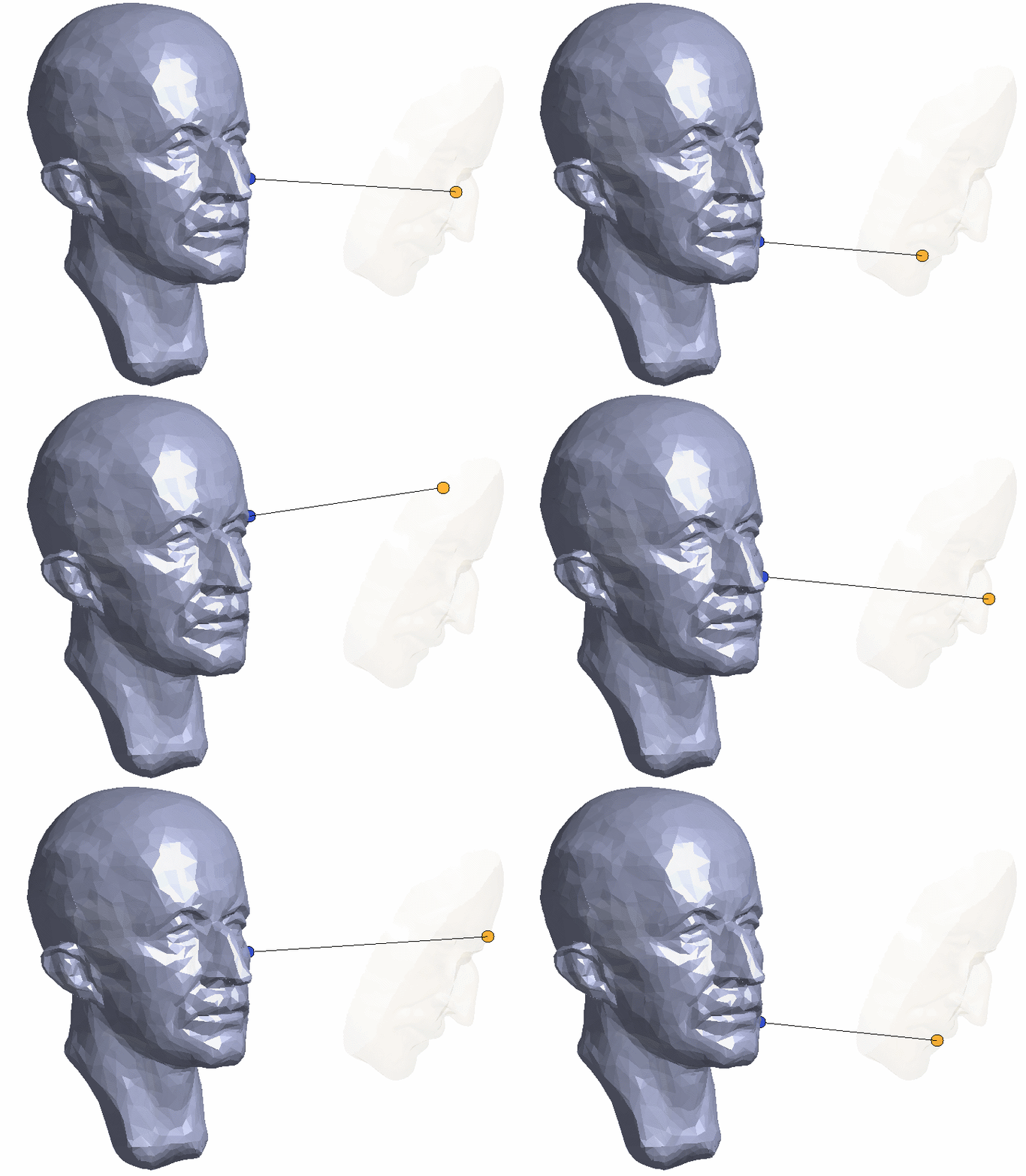
    X ← sample source mesh (V_X,F_X)
    P0 ← project all X onto target mesh (V_Y,F_Y)
    R,t ← update rigid transform to best match X and P0
    V_X ← rigidly transform original source mesh by R and t

Updating the rigid transformation

We would like to find the rotation matrix $\Rot ∈ SO(3) ⊂ \R^{3×3}$ and translation vector $\t∈\R³$ that best aligns a given a set of points $\X ∈ \R^{k×3}$ on the source mesh and their current closest points $\P ∈ \P^{k×3}$ on the target mesh. We have two choices for linearizing our matching energy: point-to-point (gradient descent) and point-to-plane (Gauss-Newton).

In either case, this is still a non-linear optimization problem. This time due to the constraints rather than the energy term.

We require that $\Rot$ is not just any 3×3 matrix, but a rotation matrix. We can linearize this constraint, by assuming that the rotation in $\Rot$ will be very small and thus well approximated by the identity matrix $\I$ plus a skew-symmetric matrix:

\[ \Rot \approx \I + \left(\begin{array}{ccc} 0 & -γ & β \ γ & 0 & -α \ -β & α & 0 \ \end{array}\right) \]

where we can now work directly with the three scalar unknowns $α$, $β$ and $γ$.

Approximate point-to-point minimizer

If we apply our linearization of $\Rot$ to the point-to-point distance linearization of the matching energy, our minimization becomes:

\[ \mathop{\text{minimize}}{\t∈\R³, α, β, γ} ∑{i=1}^k \left| \left(\begin{array}{ccc} 0 & -γ & β \ γ & 0 & -α \ -β & α & 0 \ \end{array}\right) \x_i + \t - \p_i \right|^2. \]

This energy is quadratic in the translation vector $\t$ and the linearized rotation angles $α$, $β$ and $γ$. Let's gather these degrees of freedom into a vector of unknowns: $\u = [α β γ \t^\transpose] ∈ \R⁶$. Then we can write our problem in summation form as:

\[ \mathop{\text{minimize}}{\u∈\R⁶} ∑{i=1}^k \left| \left(\begin{array}{cccccc} 0 & x_{i,3} & -x_{i,2} & 1 & 0 & 0 \ -x_{i,3} & 0 & x_{i,1} & 0 & 1 & 0 \ x_{i,2} & -x_{i,1} & 0 & 0 & 0 & 1 \end{array}\right) \u + \x_i - \p_i \right|^2. \]

This can be written compactly in matrix form as:

\[ \mathop{\text{minimize}}{\u∈\R⁶} \left| \underbrace{ \left(\begin{array}{cccccc} 0 & \X_3 & -\X_2 & \One & 0 & 0 \ -\X_3 & 0 & \X_1 & 0 & \One & 0 \ \X_2 & -\X_1 & 0 & 0 & 0 & \One \end{array}\right) }{\A} \u + \left[\begin{array}{c} \X_1-\P_1 \ \X_2-\P_2 \ \X_3-\P_3 \end{array}\right] \right|_F^2, \] where we introduce the matrix $\A ∈ \R^{3k × 6}$ that gathers the columns $\X_i$ of $\X$ and columns of ones $\One ∈ \R^k$.

This quadratic energy is minimized with its partial derivatives with respect to entries in $\u$ are all zero:

\[ \begin{align} \A^\transpose \A \u & = -\A^\transpose \left[\begin{array}{c} \X_1-\P_1 \ \X_2-\P_2 \ \X_3-\P_3 \end{array}\right] , \ \u & = \left(\A^\transpose \A\right)^{-1} \left(-\A^\transpose \left[\begin{array}{c} \X_1-\P_1 \ \X_2-\P_2 \ \X_3-\P_3 \end{array}\right] \right), \end{align} \]

Solving this small 6×6 system gives us our translation vector $\t$ and the linearized rotation angles $α$, $β$ and $γ$. If we simply assign

\[ \Rot ← \M := \I + \left(\begin{array}{ccc} 0 & -γ & β \ γ & 0 & -α \ -β & α & 0 \ \end{array}\right) \]

then our transformation will not be rigid. Instead, we should project $\M$ onto the space of rotation matrices.

Recovering a pure rotation from its linearization

In an effort to provide an alternative from "Least-Squares Rigid Motion Using SVD" [Sorkine 2009], this derivation purposefully avoids the trace operator and its various nice properties.

If $α$, $β$ and $γ$ are all small, then it may be safe to interpret these values as rotation angles about the $x$, $y$, and $z$ axes respectively.

In general, it is better to find the closest rotation matrix to $\M$. In other words, we'd like to solve the small optimization problem:

\[ \Rot^* = \argmin_{\Rot ∈ SO(3)} \left| \Rot - \M \right|_F^2, \] where $|\X|F^2$ computes the squared Frobenius norm of the matrix $\X$ (i.e., the sum of all squared element values. In MATLAB syntax: sum(sum(A.^2))). We can expand the norm by taking advantage of the associativity property of the Frobenius norm: \[ \Rot^* = \argmin{\Rot ∈ SO(3)} \left| \M \right|_F^2 + \left| \Rot \right|_F^2 - 2 \left<\Rot, \M \right>_F, \] where $\left&lt;\A, \B \right&gt;_F$ is the Frobenius inner product of $\A$ and $\B$ (i.e., the sum of all per-element products. In MATLAB syntax: sum(sum(A.*B))). We can drop the Frobenius norm of $\M$ term ($\left| \M \right|_F^2$) because it is constant with respect to the unknown rotation matrix $\Rot$. We can also drop the Frobenius norm of $\Rot$ term because it must equal one ($\left| \Rot\right|F^2 = 1$) since $\Rot$ is required to be a orthonormal matrix ($\Rot ∈ SO(3)$). We can drop the factor of $2$ and flip the minus sign to change our minimization problem into a maximization problem: \[ \Rot^* = \argmax{\Rot ∈ SO(3)} \left<\Rot, \M \right>_F \]

We now take advantage of the singular value decomposition of $\M = \U Σ \V^\transpose$, where $\U, \V ∈ \R^{3×3}$ are orthonormal matrices and $Σ∈\R^{3×3}$ is a non-negative diagonal matrix:

\[ \Rot^* = \argmax_{\Rot ∈ SO(3)} \left<\Rot,\U Σ \V^\transpose \right>_F. \]

The Frobenius inner product will let us move the products by $\V$ and $\U$ from the right argument to the left argument:

Recall some linear algebra properties:

1. Matrix multiplication (on the left) can be understood as acting on each column: $\A \B = \A [\B_1 \ \B_2 \ … \ \B_n] = [\A \B_1 \ \A \B_2 \ …
   \A \B_n]$,
2. The Kronecker product $\I ꕕ \A$ of the identity matrix $\I$ of size $k$ and a matrix $\A$ simply repeats $\A$ along the diagonal k times. In MATLAB, repdiag(A,k),
3. Properties 1. and 2. imply that the vectorization of a matrix product $\B\C$ can be written as the Kronecker product of the #-columns-in-$\C$ identity matrix and $\B$ times the vectorization of $\C$: $\text{vec}(\B\C) = (\I ꕕ \B)\text{vec}(\C)$,
4. The transpose of a Kronecker product is the Kronecker product of transposes: $(\A ꕕ \B)^\transpose = \A^\transpose ꕕ \B^\transpose$,
5. The Frobenius inner product can be written as a dot product of vectorized matrices: $&lt;\A,\B&gt;_F = \text{vec}(\A) ⋅ \text{vec}(\B) = \text{vec}(\A)^\transpose \text{vec}(\B)$,
6. Properties 3., 4., and 5. imply that Frobenius inner product of a matrix $\A$ and the matrix product of matrix $\B$ and $\C$ is equal to the Frobenius inner product of the matrix product of the transpose of $\B$ and $\A$ and the matrix $\C$: $&lt;\A,\B\C&gt;_F = \text{vec}(\A)^\transpose \text{vec}(\B\C) = \text{vec}(\A)^\transpose (\I ꕕ \B)\text{vec}(\C) = \text{vec}(\A)^\transpose (\I ꕕ \B^\transpose)^\transpose \text{vec}(\C) = \text{vec}(\B^\transpose\A)^\transpose \text{vec}(\C) = &lt;\B^\transpose \A,\C&gt;_F$.

\[ \Rot^* = \argmax_{\Rot ∈ SO(3)} \left<\U^\transpose \Rot \V, Σ \right>_F. \]

Now, $\U$ and $\V$ are both orthonormal, so multiplying them against a rotation matrix $\Rot$ does not change its orthonormality. We can pull them out of the maximization if we account for the reflection they might incur: introduce $Ω = \U^T\Rot\V ∈ O(3)$ with $\det{Ω} = \det{\U\V^\transpose}$. This implies that the optimal rotation for the original probklem is recovered via $\Rot^* = \U Ω^* \V^\transpose$. When we move the $\argmax$ inside, we now look for an orthonormal matrix $Ω ∈ O(3)$ that is a reflection (if $\det{\U\V^\transpose} = -1$) or a rotation (if $\det{\U\V^\transpose} = 1$):

\[ \Rot^* = \U \left( \argmax_{Ω ∈ O(3),\ \det{Ω} = \det{\U\V^\transpose}} \left<Ω, Σ \right>_F \right) \V^\transpose. \]

This ensures that as a result $\Rot^$ will be a rotation: $\det{\Rot^} = 1$.

Recall that $Σ∈\R^{3×3}$ is a non-negative diagonal matrix of singular values sorted so that the smallest value is in the bottom right corner.

Because $Ω$ is orthonormal, each column (or row) of $Ω$ must have unit norm. Placing a non-zero on the off-diagonal will get "killed" when multiplied by the corresponding zero in $Σ$. So the optimal choice of $Ω$ is to set all values to zero except on the diagonal. If $\det{\U\V^\transpose} = -1$, then we should set one (and only one) of these values to $-1$. The best choice is the bottom right corner since that will multiply against the smallest singular value in $∑$ (add negatively affect the maximization the least):

\[ Ω^*_{ij} = \begin{cases} 1 & \text{ if $i=j\lt3$} \\ \det{\U\V^\transpose} & \text{ if $i=j=3$} \\ 0 & \text{ otherwise.} \end{cases} \]

Finally, we have a formula for our optimal rotation:

\[ \Rot = \U Ω^* \V^\transpose. \]

Closed-form point-to-point minimizer

Interestingly, despite the non-linear constraint on $\Rot$ there is actually a closed-form solution to the point-to-point matching problem:

\[ \mathop{\text{minimize}}{\t∈\R³,\ \Rot ∈ SO(3)} ∑{i=1}^k ‖\Rot \x_i + \t - \p_i‖², \]

This is a variant of what's known as a Procrustes problem, named after a mythical psychopath who would kidnap people and force them to fit in his bed by stretching them or cutting off their legs. In our case, we are forcing $\Rot$ to be perfectly orthogonal (no "longer", no "shorter).

Substituting out the translation terms

This energy is quadratic in $\t$ and there are no other constraints on $\t$. We can immediately solve for the optimal $\t^*$---leaving $\Rot$ as an unknown---by setting all derivatives with respect to unknowns in $\t$ to zero:

\[ \begin{align} \t^* &= \argmin_{\t} ∑_{i=1}^k ‖\Rot \x_i + \t - \p_i‖² \\ &= \argmin_\t \left|\Rot \X^\transpose + \t \One^\transpose - \P^\transpose\right|^2_F, \end{align} \] where $\One ∈ \R^{k}$ is a vector ones. Setting the partial derivative with respect to $\t$ of this quadratic energy to zero finds the minimum: \[ \begin{align} 0 &= \frac{∂}{∂\t} \left|\Rot \X^\transpose + \t \One^\transpose - \P^\transpose\right|^2_F \\ &= \One^\transpose \One \t + \Rot \X^\transpose \One - \P^\transpose \One, \end{align} \]

Rearranging terms above reveals that the optimal $\t$ is the vector aligning the centroids of the points in $\P$ and the points in $\X$ rotated by the---yet-unknown---$\Rot$. Introducing variables for the respective centroids $\hat{\p} = \tfrac{1}{k} ∑_{i=1}^k \p_i$ and $\hat{\x} = \tfrac{1}{k} ∑_{i=1}^k \x_i$, we can write the formula for the optimal $\t$:

\[ \begin{align} \t &= \frac{\P^\transpose \One - \Rot \X^\transpose \One}{ \One^\transpose \One} \\ &= \hat{\p} - \Rot \hat{\x}. \end{align} \]

Now we have a formula for the optimal translation vector $\t$ in terms of the unknown rotation $\Rot$. Let us substitute this formula for all occurrences of $\t$ in our energy written in its original summation form:

\[ \mathop{\text{minimize}}{\Rot ∈ SO(3)} ∑\limits{i=1}^k \left| \Rot \x_i + ( \hat{\p} - \Rot\hat{\x}) - \p_i \right|^2 \
\mathop{\text{minimize}}{\Rot ∈ SO(3)} ∑\limits{i=1}^k \left| \Rot (\x_i - \hat{\x}) - (\p_i - \hat{\p}) \right|^2 \\ \mathop{\text{minimize}}{\Rot ∈ SO(3)} ∑\limits{i=1}^k \left| \Rot \overline{\x}_i - \overline{\p}i \right|^2 \\ \mathop{\text{minimize}}{\Rot ∈ SO(3)} \left| \Rot \overline{\X}^\transpose - \overline{\P}^\transpose \right|_F^2, \]

where we introduce $\overline{\X} ∈ \R^{k × 3}$ where the ith row contains the relative position of the ith point to the centroid $\hat{\x}$: i.e., $\overline{\x}_i = (\x_i - \hat{\x})$ (and analagously for $\overline{\P}$).

Now we have the canonical form of the orthogonal procrustes problem. To find the optimal rotation matrix $\Rot^*$ we will massage the terms in the minimization until we have a maximization problem involving the Frobenius inner-product of the unknown rotation $\Rot$ and covariance matrix of $\X$ and $\P$:

\[ \begin{align} \Rot^* &= \argmin_{\Rot ∈ SO(3)} \left| \Rot \overline{\X}^\transpose - \overline{\P}^\transpose \right|F^2 \\ &= \argmin{\Rot ∈ SO(3)} \left<\Rot \overline{\X}^\transpose - \overline{\P}^\transpose , \Rot \overline{\X}^\transpose - \overline{\P}^\transpose \right>F\\ &= \argmin{\Rot ∈ SO(3)} \left| \overline{\X} \right|_F^2 + \left| \overline{\P} \right|_F^2 - 2 \left<\Rot \overline{\X}^\transpose , \overline{\P}^\transpose \right>F\\ &= \argmax{\Rot ∈ SO(3)} \left<\Rot,\overline{\P}^\transpose,\overline{\X}\right>F\\ &= \argmax{\Rot ∈ SO(3)} \left<\Rot,\M\right>_F\ \end{align} \]

Letting $\M = \overline{\P}^\transpose,\overline{\X}$ we can now follow the steps above using singular value decomposition to find the optimal $\Rot$.

Approximate point-to-plane minimizer

If we apply our linearization of $\Rot$ to the point-to-plane distance linearization of the matching energy, our minimization is:

\[ \mathop{\text{minimize}}{\t∈\R³, α, β, γ} ∑{i=1}^k \left( \left( \left(\begin{array}{ccc} 0 & -γ & β \ γ & 0 & -α \ -β & α & 0 \ \end{array}\right)\x_i + \x_i + \t - \p_i \right)⋅\n_i \right)^2. \]

We can follow similar steps as above. Let's gather a vector of unknowns: $\u = [α β γ \t^\transpose] ∈ \R⁶$. Then we can write our problem in summation form as:

\[ \mathop{\text{minimize}}{\u∈\R⁶} ∑{i=1}^k \left(\n_i^\transpose \left(\begin{array}{cccccc} 0 & x_{i,3} & -x_{i,2} & 1 & 0 & 0 \ -x_{i,3} & 0 & x_{i,1} & 0 & 1 & 0 \ x_{i,2} & -x_{i,1} & 0 & 0 & 0 & 1 \end{array}\right) \u + \n_i^\transpose(\x_i - \p_i) \right)^2. \]

This can be written compactly in matrix form as:

\[ \mathop{\text{minimize}}_{\u∈\R⁶} \left( \left[\begin{array}{ccc} \text{diag}(\N_1) & \text{diag}(\N_2) & \text{diag}(\N_2)\end{array}\right] \left( \A \u + \left[\begin{array}{c} \X_1-\P_1 \ \X_2-\P_2 \ \X_3-\P_3 \end{array}\right]\right) \right)^2, \]

where $\N_i$ is the ith column from the matrix of normals $\N ∈ \R^{k × 3}$, $\text{diag}(\v)$ creates a diagonal matrix from a vector, and $\A ∈ \R^{3k × 6}$ is the same as above.

This energy is quadratic in $\u$ and can be solve by setting all partial derivatives with respect to $\u$ to zero.

Closed-form point-to-point minimizer

To the best of my knowledge, no known closed-form solution exists. I am not sure whether it can not exist or just whether no one has figured it out (or they did and I just do not know about it).

Uniform random sampling of a triangle mesh

Our last missing piece is to sample the surface of a triangle mesh $X$ with $m$ faces uniformly randomly. This allows us to approximate continuous integrals over the surface $X$ with a summation of the integrand evaluated at a finite number of randomly selected points. This type of numerical integration is called the Monte Carlo method.

We would like our random variable $\x ∈ X$ to have a uniform probability density function $f(\x) = 1/A_X$, where $A_X$ is the surface area of the triangle mesh $X$. We can achieve this by breaking the problem into two steps: uniformly sampling in a single triangle and sampling triangles non-uniformly according to their area.

Suppose we have a way to evaluate a continuous random point $\x$ in a triangle $T$ with uniform probability density function $g_T(\x) = 1/A_T$ and we have a away to evaluate a discrete random triangle index $T ∈ {1,2,‥,m}$ with discrete probability distribution $h(T) = A_T/A_X$, then the joint probability of evaluating a certain triangle index $T$ and then uniformly random point in that triangle $\x$ is indeed uniform over the surface:

\[ h(T) g_T(\x) = \frac{A_T}{A_X} \frac{1}{A_T} = \frac{1}{A_X} = f(\x). \]

Uniform random sampling of a single triangle

In order to pick a point uniformly randomly in a triangle with corners $\v_1, \v_2, \v_3 ∈ \R^3$ we will first pick a point uniformly randomly in the parallelogram formed by reflecting $\v_1$ across the line $\overline{\v_2\v_3}$:

\[ \x = \v_1 + α (\v_2-\v_1) + β (\v_3 - \v_1) \]

where $α,β$ are uniformly sampled from the unit interval $[0,1]$. If $α+β &gt; 1$ then the point $\x$ above will lie in the reflected triangle rather than the original one. In this case, preprocess $α$ and $β$ by setting $α←1-α$ and $β←1-β$ to reflect the point $\x$ back into the original triangle.

Area-weighted random sampling of triangles

Assuming we know how to draw a continuous uniform random variable $γ$ from the unit interval $[0,1]$, we would now like to draw a discrete random triangle index $T$ from the sequence ${1,‥,m}$ with likelihood proportional to the relative area of each triangle in the mesh.

We can achieve this by first computing the cumulative sum $\C ∈ \R^{m}$ of the relative areas:

\[ C_i = ∑_{j=1}^i \frac{A_j}{A_X}, \]

Then our random index is found by identifying the first entry in $\C$ whose value is greater than a uniform random variable $γ$. Since $\C$ is sorted, locating this entry can be done in $O(\log m)$ time.

Why is my code so slow?

Try profiling your code. Where is most of the computation time spent?

If you have done things right, the majority of time is spent computing point-to-mesh distances. For each query point, the computational complexity of computing its distance to a mesh with $m$ faces is $O(m)$.

This can be dramatically improved (e.g., to $O(\log m)$ on average) using an space partitioning data structure such as a kd tree, a bounding volume hierarchy, or spatial hash.

Tasks

Read [Bouaziz 2015]

This reading task is not directly graded, but it's expected that you read and understand sections 3.2-3.3 of Sofien Bouaziz's PhD thesis "Realtime Face Tracking and Animation" 2015. Understanding this may require digging into wikipedia, other online resources or other papers.

Blacklist

You may not use the following libigl functions:

• igl::AABB
• igl::fit_rotations
• igl::hausdorff
• igl::point_mesh_squared_distance
• igl::point_simplex_squared_distance
• igl::polar_dec
• igl::polar_svd3x3
• igl::polar_svd
• igl::random_points_on_mesh

Whitelist

You are encouraged to use the following libigl functions:

• igl::cumsum computes cumulative sum
• igl::doublearea computes triangle areas
• igl::per_face_normals computes normal vectors for each triangle face

src/random_points_on_mesh.cpp

Generate n random points uniformly sampled on a given triangle mesh with vertex positions VX and face indices FX.

src/point_triangle_distance.cpp

Compute the distance d between a given point x and the closest point p on a given triangle with corners a, b, and c.

src/point_mesh_distance.cpp

Compute the distances D between a set of given points X and their closest points P on a given mesh with vertex positions VY and face indices FY. For each point in P also output a corresponding normal in N.

It is OK to assume that all points in P lie inside (rather than exactly at vertices or exactly along edges) for the purposes of normal computation in N.

src/hausdorff_lower_bound.cpp

Compute a lower bound on the directed Hausdorff distance from a given mesh (VX,FX) to another mesh (VY,FY). This function should be implemented by randomly sampling the $X$ mesh.

src/closest_rotation.cpp

Given a 3×3 matrix M, find the closest rotation matrix R.

src/point_to_point_rigid_matching.cpp

Given a set of source points X and corresponding target points P, find the optimal rigid transformation (R,t) that aligns X to P, minimizing the point-to-point matching energy.

You may implement either that "Approximate" solution via linearizing the rotation matrix or the "closed form" solution

src/point_to_plane_rigid_matching.cpp

Given a set of source points X and corresponding target points P and their normals N, find the optimal rigid transformation (R,t) that aligns X to planes passing through P orthogonal to N, minimizing the point-to-point matching energy.

src/icp_single_iteration.cpp

Conduct a single iteration of the iterative closest point method align (VX,FX) to (VY,FY) by finding the rigid transformation (R,t) minimizing the matching energy.

The caller can specify the number of samples num_samples used to approximate the integral over $X$ and specify the method (point-to-point or point-to-plane).