BIAS EVALUATION FOR MODELS OF TOXIC CONVERSATIONS CLASSIFICATION
Abstract
This project proposes to implement, as part of a Kaggle competition, a metric to evaluate a machine learning algorithm operating on a population composed of individuals classified in subgroups. These subgroups mark a social or ethnic identity of the individuals making up the population.
Details of projects : https://www.kaggle.com/c/jigsaw-unintended-bias-in-toxicity-classification
An exploratory analysis of the corpus of texts has been conducted allowing to argue over the choice of learning model.
Data-preparation process is described and leads to a digital representation of the input data to feed machine learning algorithm.
The study of machine learning hyper-parameters is conducted and parameters used for building learning model are selected.
Selected model is trained and results in term of binary classifications are exposed along with bias computation in compliance with formula described in https://www.kaggle.com/c/jigsaw-unintended-bias-in-toxicity-classification/overview/evaluation
Software architecture
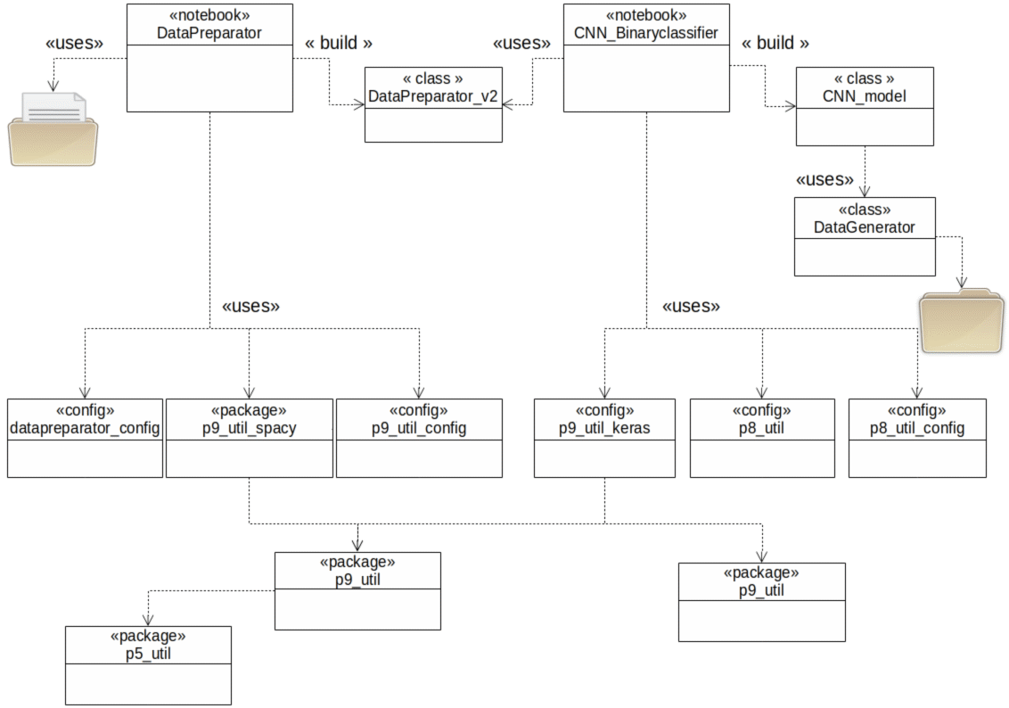
This software architecture is drawned with UML syntax. It is organized as layers of packages issued from other Data Sciences projects. They are reused here to face effectiveness, productitivy and quality issues.
All packages are implemented with Python 3.6 language.Architecture semantic is interpreted as following :
- The notebook DataPreparator.ipynb uses file where dataset is stored in to read it.
-
The notebook CNN_BinaryClassifier.ipynb uses DataPreparator_v2 Python object in order to build a Keras CNN model for binary classification. This model is saved on harddisk into a H5 format.
-
The CNN model uses an instance of DataGenerator.py class in order to access data in a bulk way. Data is stored in a folder of hardisk. This allows to save memory ressources, using hardisk as a memory ressource extension and also to train model with cross-validations over K-folds datasets.
Exploratory analyis
Features description
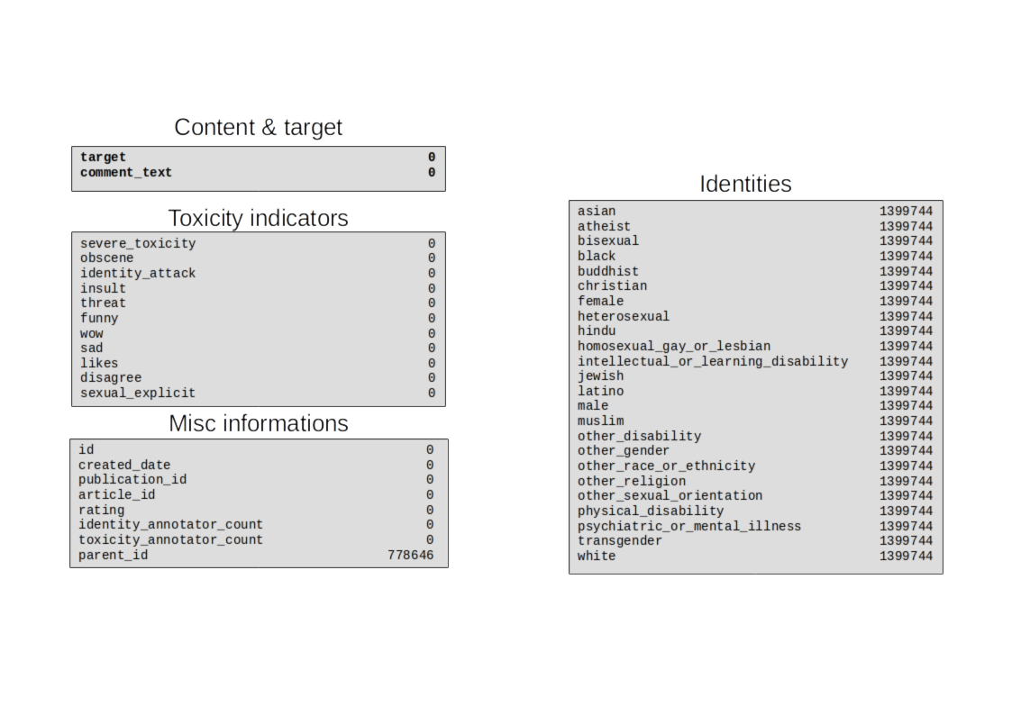
* Dataset features identification*The dataset is composed of 45 columns described as following:
-
Toxicity indicators : these features indicates the type of toxicity
-
Identities : these features indicates presence into comments of words or expressions related to an identity. Bias of predictive model will be evaluate against some of these identities.
-
Misc informations : these features provide additional informations over comments.
-
Content & target : Content are used to feed machine learning model (after a data-preparation and a digitalization process) and target are used as labels to train models.
Target distribution
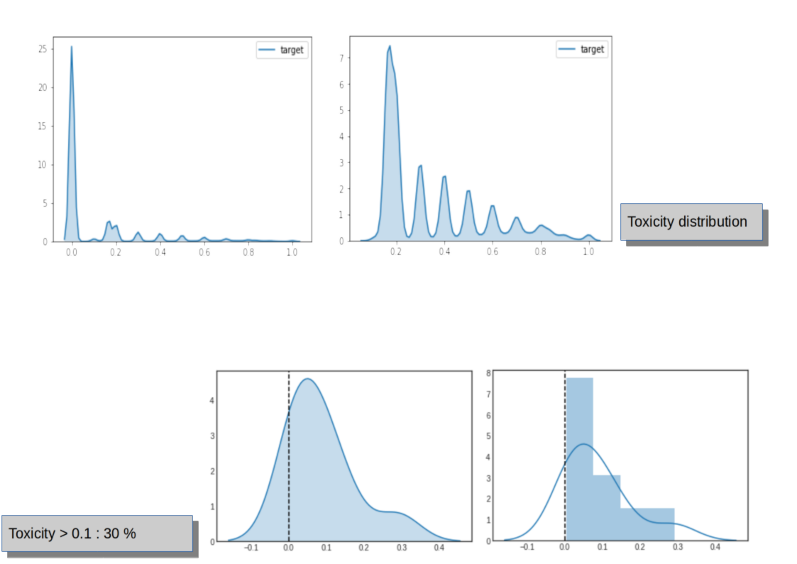
* Toxiciy distribution over the dataset*Toxicity values (named target) are ranged from 0.0 (safe comment) to 1.0 (more toxic comment).
Toxicity disrtribution shows unbalanced classes. Around 30% of comments have a toxicity value greater then 0.0.
Note also that continuous values of toxicity are difficult to interpret and perceive distinctly for a human. E.g it is not clear to perceive how far a comment with toxicity value of 0.38 is fare from another comment with toxicity value fixed to 0.35.
Toxicity contributors analysis
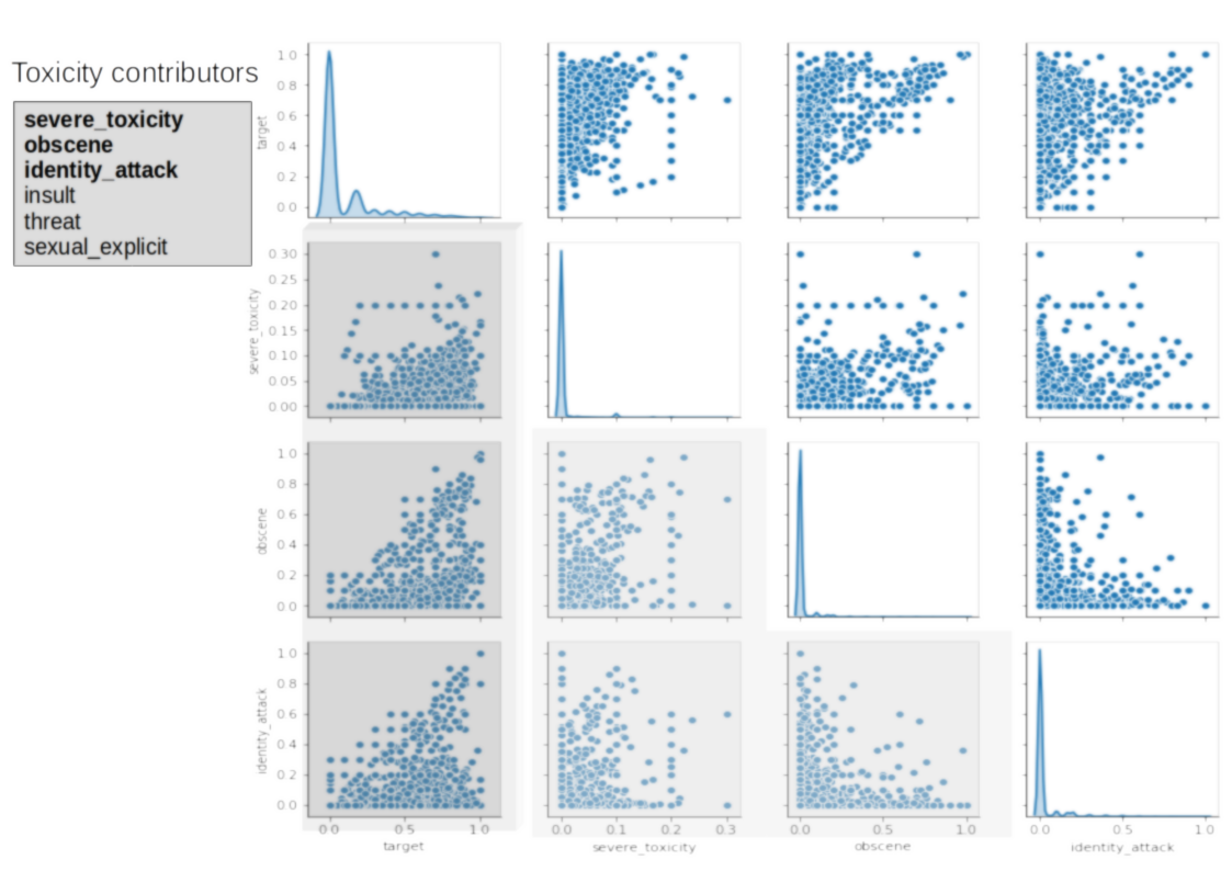
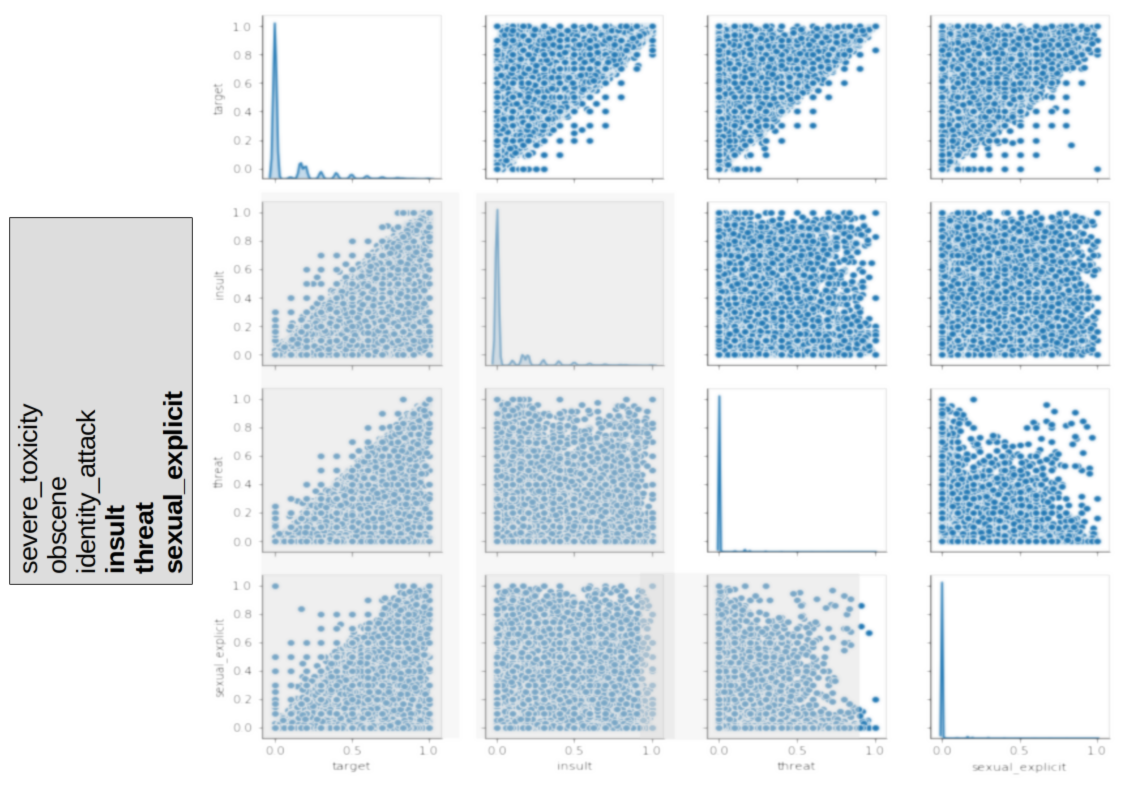
* Multi-variate analysis for toxicity contributors (1)*The group of features, named **Toxicity distribution** are analysed against target values in order to highlight associations between dependant variables and features.
This multivariate analysis shows that identity_attack, obscene and severe_toxicity in extruded area show a linear border of the shape of distributed points along with target. The border of the shape increases linearly with toxicity range of values. The fact that a dense area of points appears under the diagonal border let think that contribution to toxicity may be due to a combinaison of at least these three features.
We note also that in non extruded area, multivariate analysis between features identity_attack and obscene expose the same kind of linearly border shape that linearly decreases.
On the display above, the multivariate analysis between features insult, threat, ** sexual_explicit** and target, over the extruded area, shows a more accentuated and dense distribution of points below the diagonal border that linearly increases with target values.
ANOVA over identities
QUESTION: is it possible to infer a relation between toxicity (the target) and identities ?
Identities are used in order to evaluate bias. The idea behind, is to evaluate the existance of relations betweens various identities with toxicity level.
The bias computation process consists in defining thresholds for both, identity feature and target from which, 2 classes are defined. The bias evaluation leads to to build a binary classification algorithm. The point of interest here is to try to make sense for a fixed threshold value.
For doing so, ANOVA is applied over each one of the groups formed with identities.
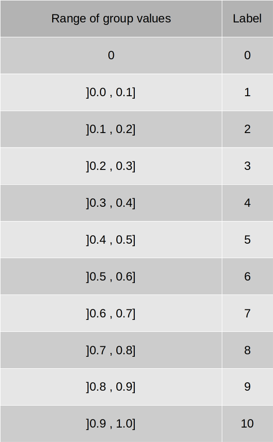
Identities values are continuous values ranged from 0.0 to 1.0. These values are reworked and are labelized with values 0,1,... 10. Such transformation allows to consider identities as formed with qualitative groups. Modalities in any group are ranged from 0 to 10. These labelized ranges of values may be interpreted as levels of the considered identity.
The labeling scheme is as following :
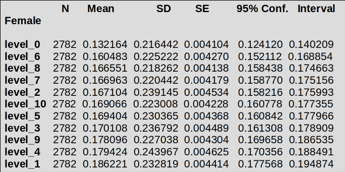
E.g. for female identity, such transformation leads to consider 11 groups, ranged from 0 to 10, with statistics values describe below for female identity :
Means values are the means of toxicity computed for each group inside comments marked with female identity. All these statistics have been computed over toxicity grouped by identities.
Question : are differences between these means significant ? Is there an inferable relation between identities labels, ranged from 0 to 10, and toxicity level of a comment ?
For any of the groups in the list above, Levene test is conducted. p-values, nearly 0, allows to invalidate homodestaticity hypothesis : variance in each group have no equal values. This is the H0 hypothesis stating over variance equality between the groups of an identity. Nevertheless, in order to balance conditions if Levene test, sampling has been processed in a such way that the number of observations into each group is same. Under this condition, ANOVA test may be conducted.
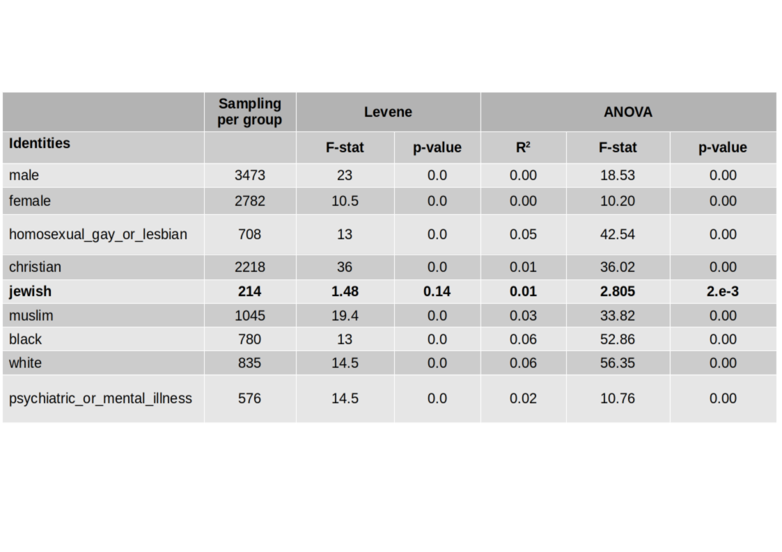
Results are produced on the figure below:
Levene test seems to be not significant for all identities except jewish group. Nevertheless, for making F-stat robust considering normality and homodestaticity hypothesis, all groups inside each one of the identities have been sampled with the same number of observations. Then, for each identity, considering F-stat magnetude (that measures a ratio of the variability of the mean inside groups and the variability of the mean between groups) and associated p-value << 5.e-2 (that indicates how significant is the result of F-stat), test over differences of means between groups are regarded as significant.
As a conclusion of ANOVA :
-
Considering
F-statvalues (variance in-between groups over within groups variance) for all identities, there is a significant difference between means of groups, groups organized as levels of an identity. -
Considering
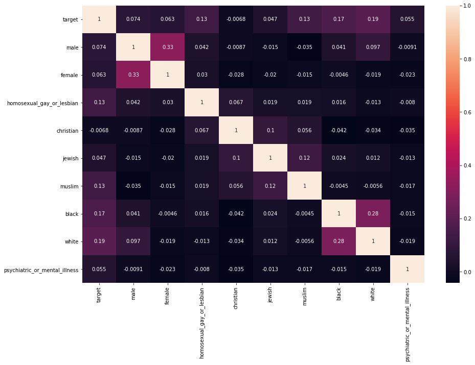
R²values for all identities, explained variance is weak for any identity (considering here as quantitative features), leading to the conclusion that none of the identities have a size effect over comments toxicity. Correlation matrix here-under partially illustrates this claims. This correlation matrix has been built over the whole observations. We note a symetrix aspect of correlations between couples of features(male, female)and(black, white). These features show a middle size effect for explaing target variance.
* Correlation matrix of identities levels*
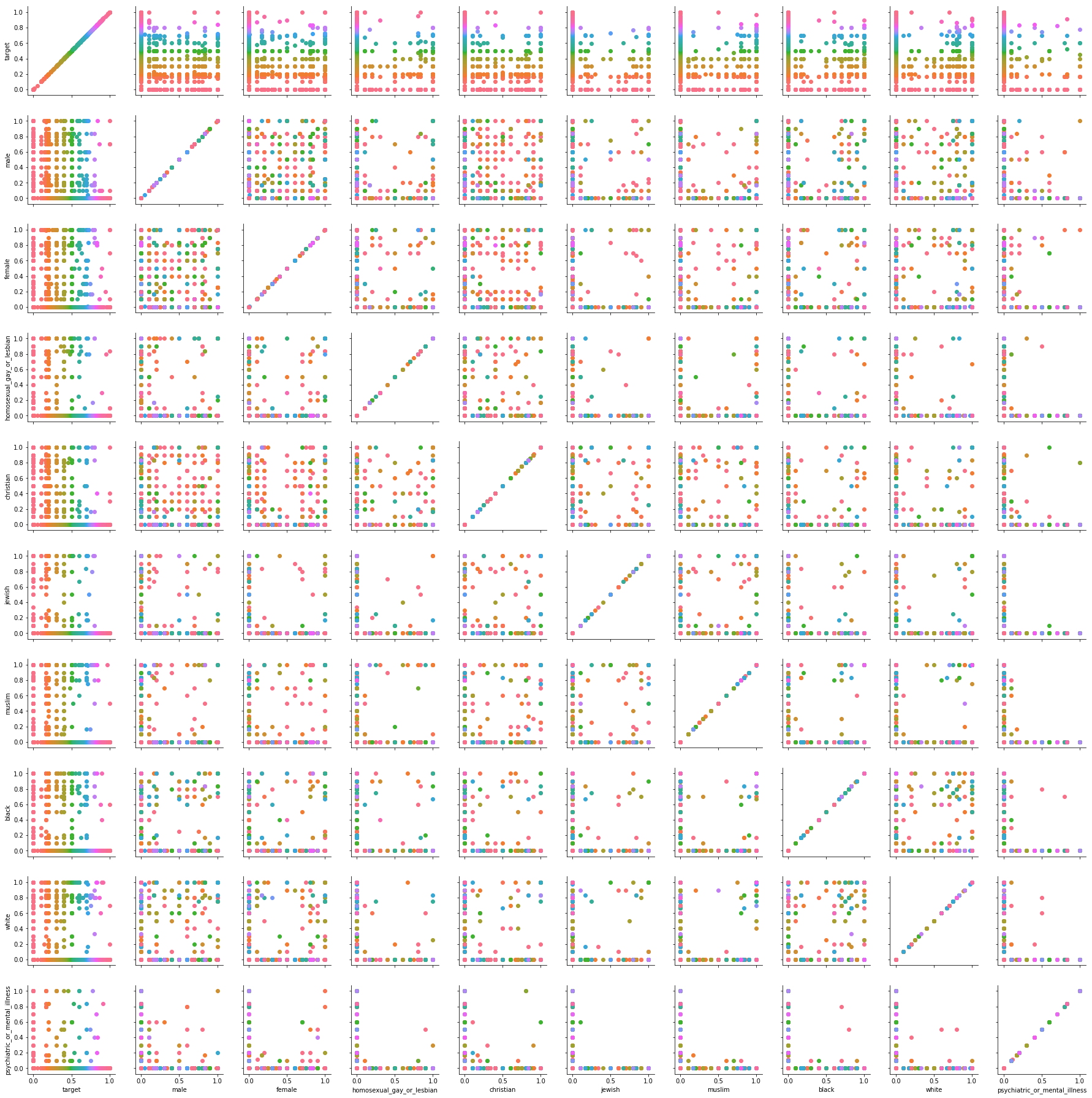
In addition, diagram belows exposes the distribution of a sample of 5000 points for identities that are taken into account for bias evaluation along with toxicity. There is no intuitive evidence of informational shape as pointed for toxicity contributors features on previous section.
Conclusions over features analysis
Features have been splitted into two categories : contributors to toxicity of coments and identities. It has been shown that contributors to toxicity have a strong effect over the toxicity magnetude, whereas identities have a weak effect over toxicity. Unintended bias in machine learning classification comes with the fact that despite that last point, comments tend to be classified as toxic when they embedd some identities terms or expressions.
Absence of identity effects over toxicity also let us think that the process involved in toxicity and identity metrics can be safely taken into account. This lead to consider as reliable comments labelization used in a supervized machine learning model.
Same remark also stands for toxicity contributors. Their co-variancy behaviour along with toxicity is compliant with the intuitive sens, stating that a comment that embbeds insulting terms or expressions is welling to render it toxic.
Proper algorithms should be able to take into account the presence of toxicity contributors along with identities in comments in order to proceed to classification.
Also, post-hoc tests shows no evidence of an existance of treshold effect identifying differences between means of different groups inside an identity.
**For the followings sections, toxicity and identities groups levels are considered as latent values that explain the variancy of target values. M.L. algorithms will only have comments as independant features and toxicity levels as targets**.
Data preparation & digitalization process
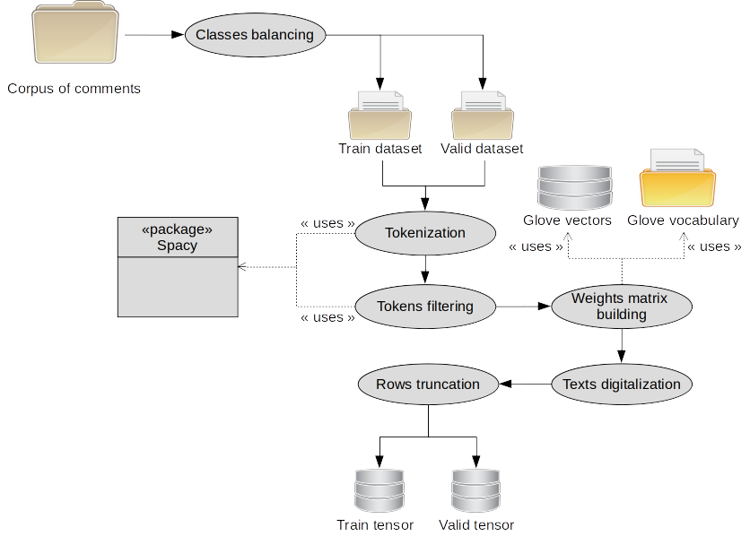
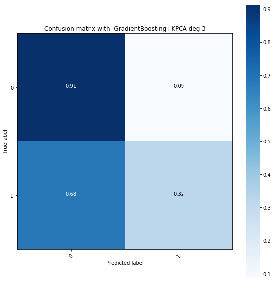
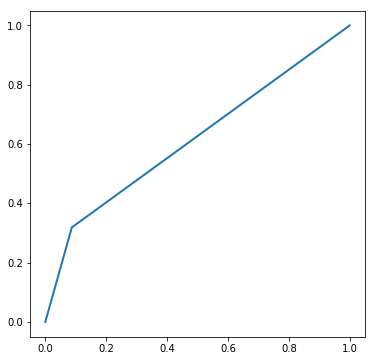
This process allows to transforms a corpus of comments into a digitalized representation, allowing to feed an algorithm. The global process is described below : * Software engineering involved into data-preparation and digitalization process *- * Spacy package is used for NLP processing. Using it, sequences of words are preserved using. * Due to toxicity distribution study in previous sections, balancing dataset is required in order to ensure toxic and non toxic comments to be processed "equaly". Otherwise, contributions to cost function will be mainly due to non toxic comments that will lead to a biased prediction model. The picture below do represents a model obtained with Gradient boosting algorithm without dataset balancing. All non toxic comments are very well classified while predictions for toxic comments are not better then random prediction leading to weak performances as shown over the RAUC curve.
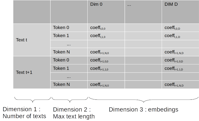
* As the result of the digitalization process, a tensor with 3 dimensions is produced, for train and validation dataset. It is represented as the figure below :
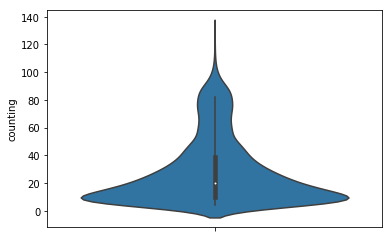
* Texts truncation : all tokenized texts should have the same number of tokens. This allows to feed NN algorithm with **same embedding layer size**. This operation takes place after the filtering process, for keeping the model with usefull informations. The max length size for the number of tokens has been fixed to 100. This value comes with the text word length distribution described on diagram below :
 Trunc of texts after digitalization allows to drive this process based on an objective criteria, such as magnetude of the vectors. Vectors with the smallest magnetude will be pushed out of digitalization representation. While doing so, relevant information that will contribute to decrease of loss function will be kept.
*   Texts padding : digitalized texts with number of tokens less then max length will be padded with zero vector.
Word embeddings
Glove allows to use different kind of model language for Naturel Language Processing. The one used here is en_core_web_lg, in which, each word in vocabulary is represented as a vector in a 300 dimensions space. Words vectors have been built using web texts and comments issued from variou social networks.
A dictionary structured as {word:glove_coefficient} is built from Glove source.
Once built, dictionary allows to build a vector for every word
in vocabulary issued from tokenizer.
Endly, weights matrix is built from vocabulary issued from tokenizer.
Such process is summarized with sequences here-under :
- * `dict_glove_word_coeff <-- processing Glove file name` * `vocabulary_word, index <-- tokenizer` * `weight_vector = dict_glove_word_coeff[vocabulary_word]` * `weight_matrix[index] = weight_vector`
Features correlations
Statistic analysis as shown that some features expose linear correlations with toxicity values.
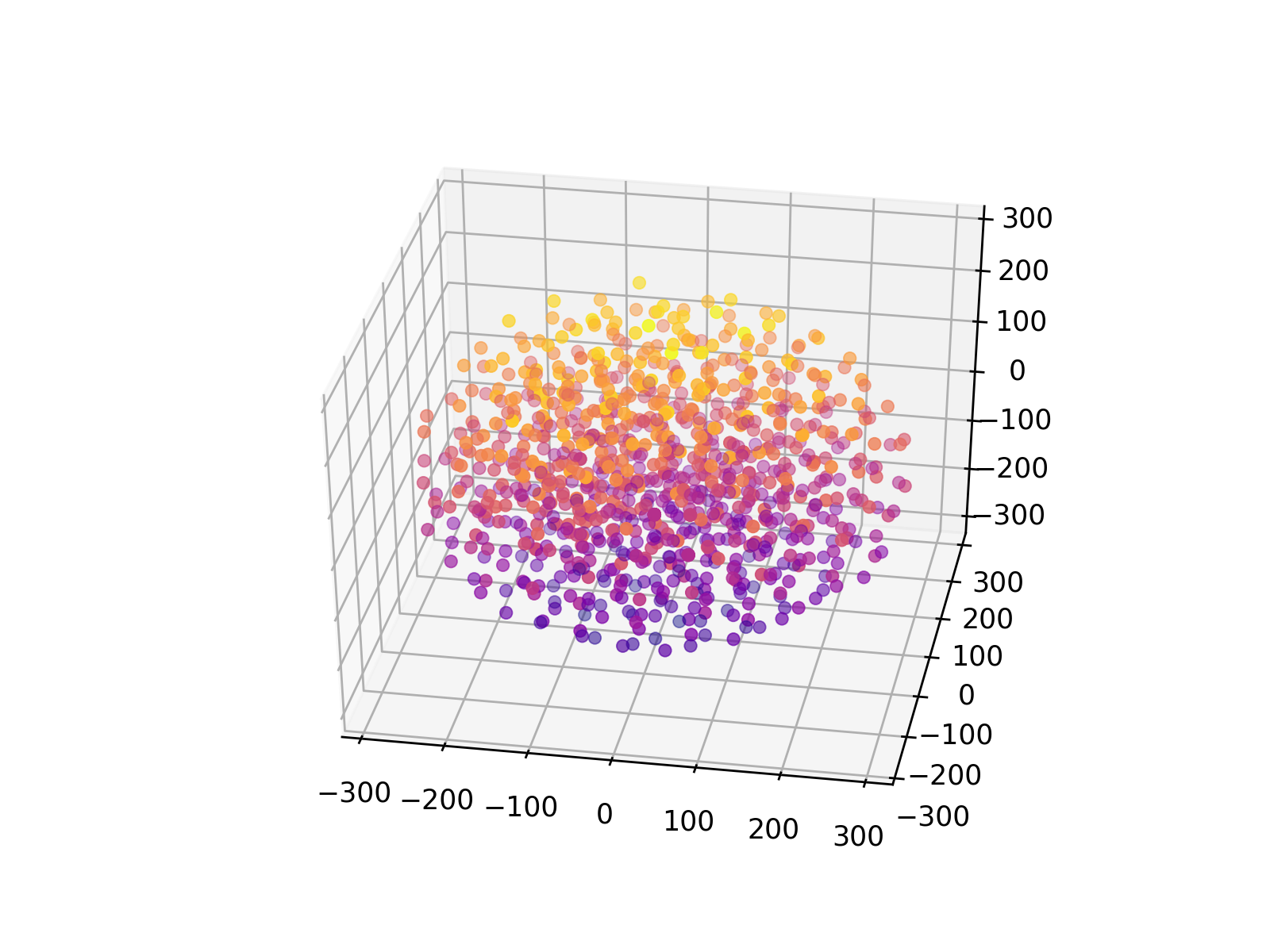
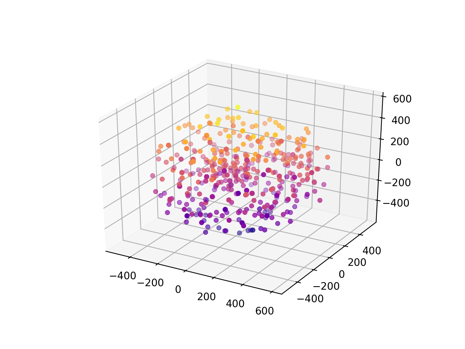
Figure below shows 1000 digitalized comments with process described in previous section. t-SNE operator is applied over 3 dimensions. There is no evidence that an hyperplan exists that is able separate groups of points. * 3D t-SNE reduction over dataset with PCA operator *
On figure below, a kernel PCA operator has been applied with kernel of order 5. The kernel trick allows to process a non linear model as a linear model in an Hilbert space of larger size then the original space.
* 3D t-SNE reduction over dataset with order 5 Kernel PCA operator *
CNN classifier
From statistic analysis conducted in previous sections, it is shown that the presence of some type of words or expressions in a comment is correlated to the toxicity level. The problem can be formulated as the way to identity in a comment, what has been named toxicity contributors and identities and relate them to a level of toxicity. Due to that, the expected prediction model should be able to learn such relations connecting identified structures with toxicity level.
The ground problem is focused on textual structures identification. CNN architectures are famous and relevant to accomplish a such task.
In addition, a bias metric defined in https://www.kaggle.com/c/jigsaw-unintended-bias-in-toxicity-classification/overview/evaluation will be applied over the model in order to evaluate how fare the model is able to distinguish toxic comments from non toxic comments that embbeds identities terms or expressions.
Rather then predict toxicity level thanks to a regression algorithm, a classifier is used to complie with the model bias evaluation.
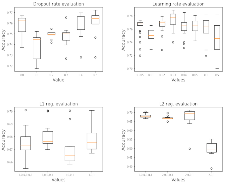
CNN hyper-parameters selection
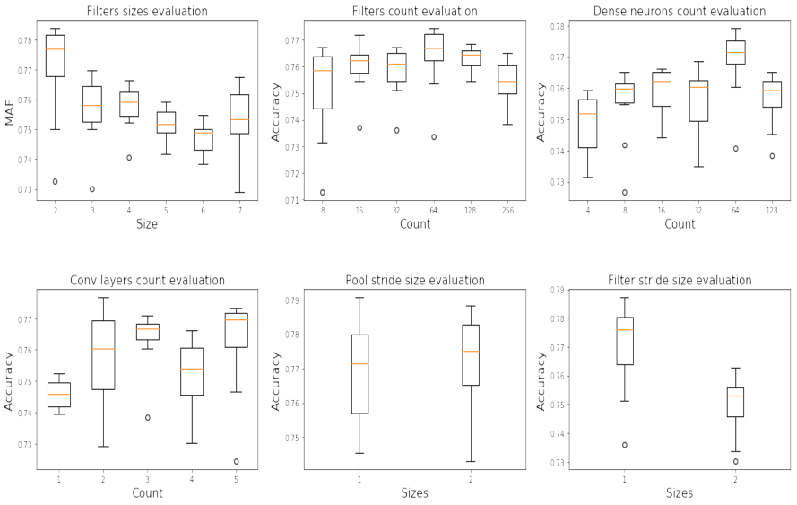
CNN hyper-parameters selection for convolutional layers
* Evaluation of hyper-parameters for convolutional layers *
These parameters are related to CNN structure :
- The size of the convolution filters. When processing text, this parameter amounts to setting n-grams for the neighborhood of words. Such a structure in word processing is related to the semantics of words, indicating that words of the same neighborhood have the same meanings.
- The number of convolutional filters, leading to features maps. This will give the model the potential for identitying all kinds of textual structures in the corpus of comments. A single feature map identifies the same structures that may be repeated in a comment.
- The number of convolutional layers.
- The filter stride size. This parameter fixes the window stride for N-GRAM structures detection.
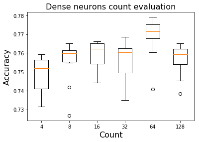
CNN hyper-parameters selection for dense layers
* Evaluation of the number of neurons into dense layer *These parameters are related to dense layers structure and they are:
-
The number of dense layers. It has been fixed to 1.
-
The number of neurons in the dense layer. Dense layers after convolutional layers allows to classify features issued from convolutional layers.
Algorithms selection :
- Gradient descent algorithm is RMSprop.
- Loss function algorithm is binary cross entropy.
CNN hyper-parameters selection for optimization :
* Hyper-parameters evaluation for model optimization *
-
Dropout rate. This parameter controls the model complexity and hence, its capacity to generalization.
-
Learning rate. This parameter controls the speed of the learning.
-
L1 regularization. This parameter controls the complexity of the algorithm, hence its bility to generalize. This regularization process is applied to the cost function. Complexity regularization is achived while killing some features in the learning process. L1 regularization is knwon to be less stable as L2 regularization, because loss function convexity is impacted with L1 terms.
-
L2 regularization. This parameter controls the complexity of the algorithm, hence its bility to generalize. This regularization process is applied to the cost function
Classification results
Binary classification
This step has been performed by spliting toxicy values into 2 classes :
- * 0.0 <= toxicity < 0.5 : safe comments * 0.5 <= toxicity <=1.0 : toxic comments
Data generators
Because of memory resources issues, DataGenerator objects have been created and used for both, trainig an validation operations.
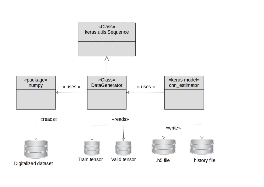
Such objects allow to pump bulk of data stored on harddisk. Architecture below shows how the model works :
DataGenerator class inherites from keras.utils.Sequence This allows Keras model to use object issued from this class as a source of data, pumping it iteration after iteration in the train or validation operations, until all data partitioned into files over hard disk have been processed.
DataGenerator is created using DataPreparator object. Such objects contains all operations for data preparation and digitalization process along with configuration parameters used inside these process. This architecture allows an automation digitalization process to take place.
Depending on object configuration, data sources may be train dataset or validation dataset. A callback function, issued from object of type keras.callbacks.ModelCheckpoint allows to save the best model issued from train operation.
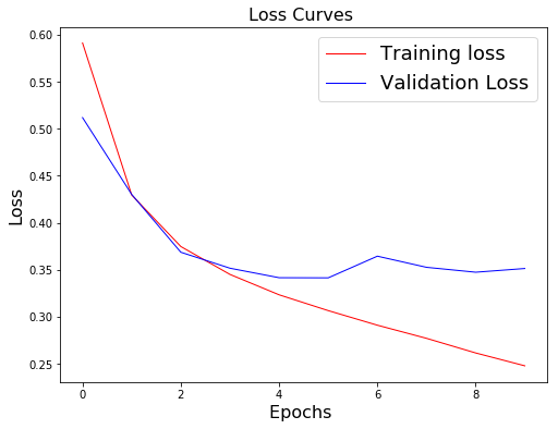
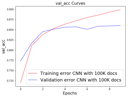
Training / validation performances
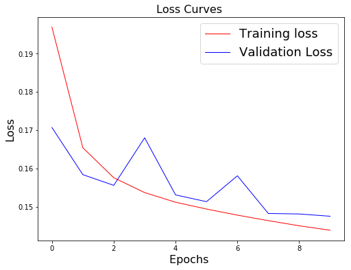
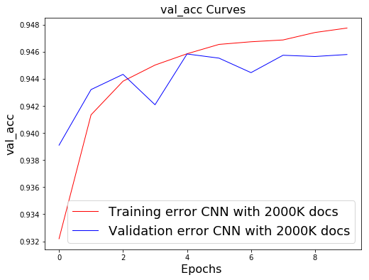
The number of trainable parameters is closed to 715K
Model tends to overfit, despites dropout rate of 0.3
Classification performances
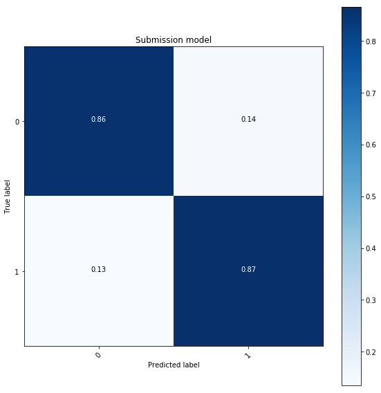
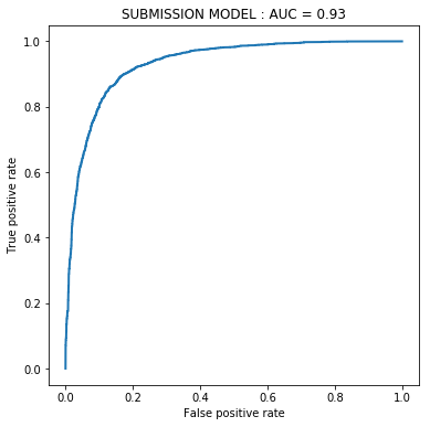
Results below have been obtained with training near to `100K` comments and validated over closed to `10K` comments. Confusion matrix below shows that model is able to properly classify :- * 86% of non toxic comments * 87% of toxic comments
Area Under RO Curve is `AUC=0.93` * Confusion matrix and ROC curve for the submission model *
Bias evaluation
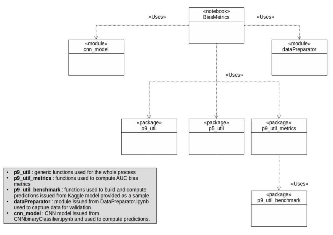
Graphic belows shows software architecture involves in the bias evaluation process.
Bias evaluation of submission model
Submission model is the one that aims to be submitted to the Kaggle competition. This is the one that has been described and built in this report.
A bias metric is defined in order to evaluate AUC over predictions, thus, for each one of the identities. For each idenity, False Positive (FP) rate and True Positive (TP) rate are jointly evaluated by defining area under ROC curve.
This metric measures three aspects of the classification for each identity :
-
BNSP_AUC: the ability of the model to distinguish safe comments without any reference (words, expressions) to the identity (such comments belongs to the group named Background Negative) from the toxic comments with reference to the identity (such comments belongs to the group named Subgroup Positive). -
BPSN_AUC: the ability of the model to distinguish toxic comments without any reference (words, expressions) to the identity (such comments belongs to the group named Background Positive) from the safe comments with references to the identity (such comments belongs to the group named Subgroup Negative). -
SUBGROUP_AUC: the ability of the model to distinguish toxic comments from non toxic comments, all comments having references to identity.
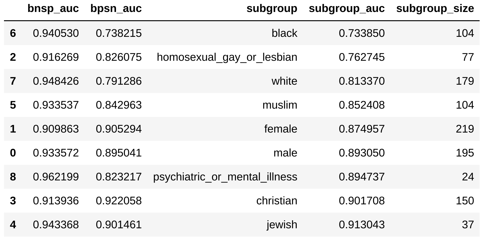
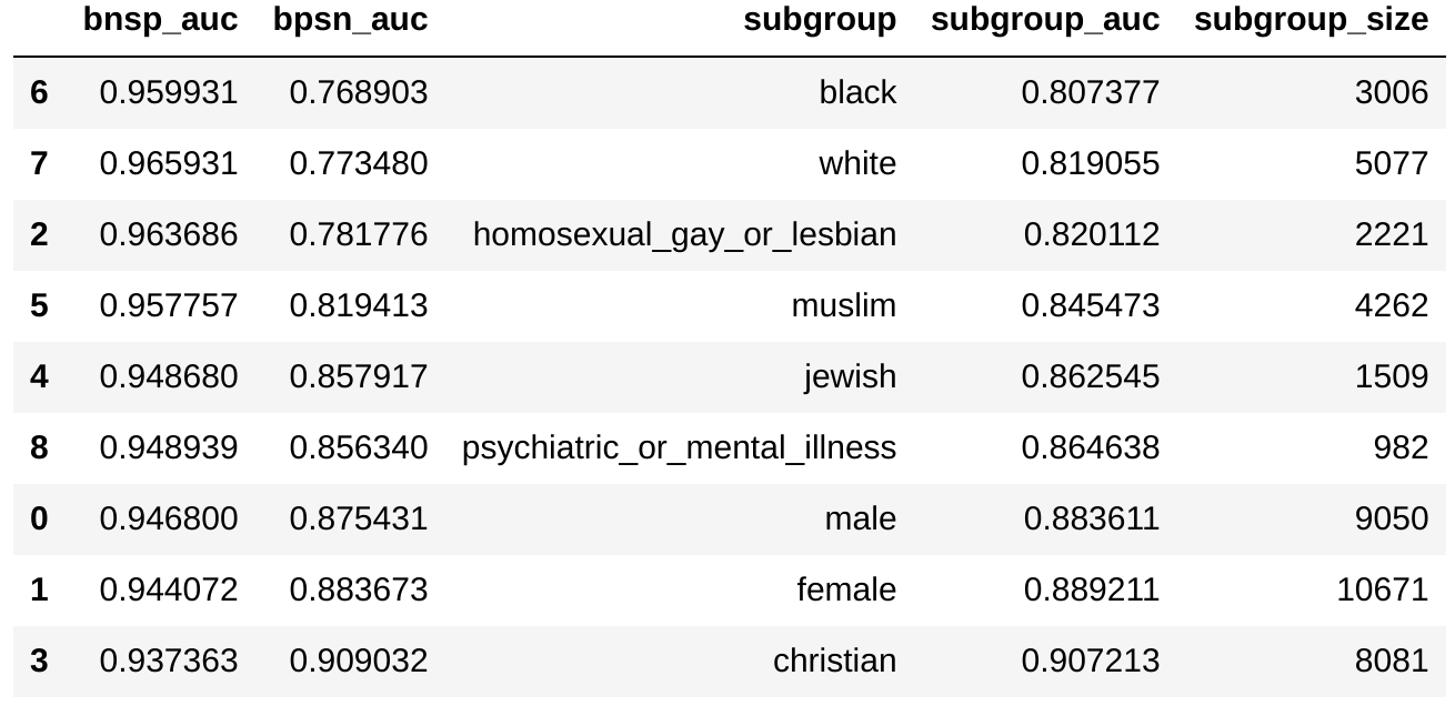
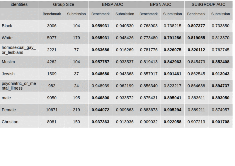
While doing so, the classification model performance is scaned for each identity. Table below shows these three values, identity per identity. * Identities AUC for the submission model *
Considering measures of `SUBGROUP_AUC`, the model confuses to distinguish toxic comments from safe one for those comments with `homosexual_gay_or_lesbian` identity. For this identity, probability that model proceeds to a proper distinction between toxic and non toxic comments in more then `75%`.
This probability of distinction is fare less then the ability of the model to distinguish from toxic comments without any reference to homosexual, gay or lebian and safe comments that contains sucg references : SUBGROUP_AUC= 0.76 < BPSN_AUC= 0.82 .
The final score is computed thanks to the overall AUC that is 0.86 and the three aspects of AUC computed separately for each identity, with the formula :
Where :
- p is the power, fixed to 5
- Ng is the number of identities involved in the bias evaluation, fixed to 9
- AUCglobal is the AUC value computed in previous section, with value=
0.86 - Other AUC values are the one extracted from bias table of identities.
- 0.25 and 0.75 are weights factors that favor ability of the model to distinguish the toxicity of texts separately for each identity over global separability ability.
For the model to be submitted to Kaggle, this formula comes with value 0.88 This may be interpreted as a bias value of 12%
Bias evaluation of benchmark model
Benchmark model is he one provided on Kaggle web site, in order to expose implementation of bias algorithm.
This is a CNN model trained with closed to 2 millions comments, say, the whole dataset. It holds close to 160K parameters.
Bias table below shows AUC values for identities :
Final score for benchmark model, measuring the bias model is 0.89
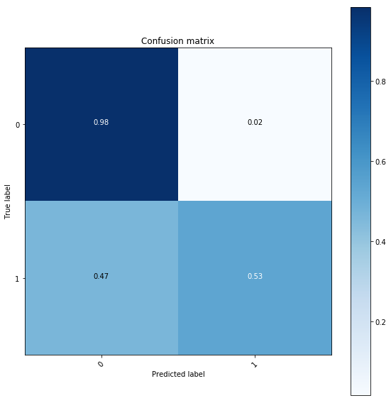
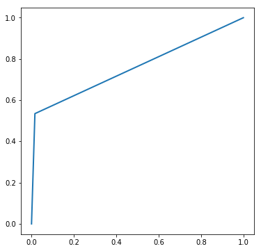
Confusion matrix below shows that, despite better performances for bias metric, benchmark model confuses more, globaly, to distinguish toxics comments from safe one, with AUC = 0.75 against 0.89 for our submission model.
Conclusions
Table below show the diffenrences of bias values between benchmark model and submission model along with identities groups with thier size used for evaluation.
Bold font shows the model with the greatest performance.Data preparation process should include emoticons.
Features may be increased with POS tags, NER, organizations tags, all such tags provided with Spacy model of language.
