 |
 |
 |
 |
 |
 |
 |
 |
 |


Heuristic Algorithms in Python
(Genetic Algorithm, Particle Swarm Optimization, Simulated Annealing, Ant Colony Algorithm, Immune Algorithm,Artificial Fish Swarm Algorithm in Python)
- Documentation: https://scikit-opt.github.io/scikit-opt/#/en/
- 文档: https://scikit-opt.github.io/scikit-opt/#/zh/
- Source code: https://github.com/guofei9987/scikit-opt
pip install scikit-optFor the current developer version:
git clone git@github.com:guofei9987/scikit-opt.git
cd scikit-opt
pip install .
All algorithms will be available on TensorFlow/Spark pytorch on version 0.4, getting parallel performance.
DE(Differential Evolution Algorithm) will be complete on version 0.5
Have fun!
UDF (user defined function) is available now!
For example, you just worked out a new type of selection function.
Now, your selection function is like this:
-> Demo code: examples/demo_ga_udf.py#s1
# step1: define your own operator:
def selection_tournament(self, tourn_size):
    FitV = self.FitV
    sel_index = []
    for i in range(self.size_pop):
        aspirants_index = np.random.choice(range(self.size_pop), size=tourn_size)
        sel_index.append(max(aspirants_index, key=lambda i: FitV[i]))
    self.Chrom = self.Chrom[sel_index, :]  # next generation
    return self.Chrom
Import and build ga
-> Demo code: examples/demo_ga_udf.py#s2
import numpy as np
from sko.GA import GA, GA_TSP

demo_func = lambda x: x[0] ** 2 + (x[1] - 0.05) ** 2 + x[2] ** 2
ga = GA(func=demo_func, n_dim=3, size_pop=100, max_iter=500, lb=[-1, -10, -5], ub=[2, 10, 2])
Regist your udf to GA
-> Demo code: examples/demo_ga_udf.py#s3
ga.register(operator_name='selection', operator=selection_tournament, tourn_size=3)scikit-opt also provide some operators
-> Demo code: examples/demo_ga_udf.py#s4
from sko.GA import ranking_linear, ranking_raw, crossover_2point, selection_roulette_2, mutation

ga.register(operator_name='ranking', operator=ranking_linear). \
    register(operator_name='crossover', operator=crossover_2point). \
    register(operator_name='mutation', operator=mutation)
Now do GA as usual
-> Demo code: examples/demo_ga_udf.py#s5
best_x, best_y = ga.run()
print('best_x:', best_x, '\n', 'best_y:', best_y)
Until Now, the udf surport
crossover,mutation,selection,rankingof GA
scikit-opt provide a dozen of operators, see here
Step1:define your problem
-> Demo code: examples/demo_ga.py#s1
import numpy as np


def schaffer(p):
    '''
    This function has plenty of local minimum, with strong shocks
    global minimum at (0,0) with value 0
    '''
    x1, x2 = p
    x = np.square(x1) + np.square(x2)
    return 0.5 + (np.sin(x) - 0.5) / np.square(1 + 0.001 * x)
Step2: do GA
-> Demo code: examples/demo_ga.py#s2
from sko.GA import GA

ga = GA(func=schaffer, n_dim=2, size_pop=50, max_iter=800, lb=[-1, -1], ub=[1, 1], precision=1e-7)
best_x, best_y = ga.run()
print('best_x:', best_x, '\n', 'best_y:', best_y)Step3: plot the result
-> Demo code: examples/demo_ga.py#s3
import pandas as pd
import matplotlib.pyplot as plt

Y_history = pd.DataFrame(ga.all_history_Y)
fig, ax = plt.subplots(2, 1)
ax[0].plot(Y_history.index, Y_history.values, '.', color='red')
Y_history.min(axis=1).cummin().plot(kind='line')
plt.show()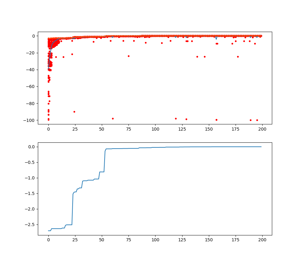
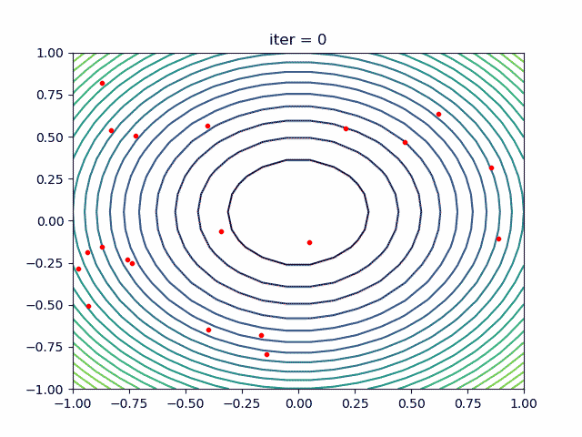
Just import the GA_TSP, it overloads the crossover, mutation to solve the TSP
Step1: define your problem. Prepare your points coordinate and the distance matrix.
Here I generate the data randomly as a demo:
-> Demo code: examples/demo_ga_tsp.py#s1
import numpy as np
from scipy import spatial
import matplotlib.pyplot as plt

num_points = 8

points_coordinate = np.random.rand(num_points, 2)  # generate coordinate of points
distance_matrix = spatial.distance.cdist(points_coordinate, points_coordinate, metric='euclidean')


def cal_total_distance(routine):
    '''The objective function. input routine, return total distance.
    cal_total_distance(np.arange(num_points))
    '''
    num_points, = routine.shape
    return sum([distance_matrix[routine[i % num_points], routine[(i + 1) % num_points]] for i in range(num_points)])
Step2: do GA
-> Demo code: examples/demo_ga_tsp.py#s2
from sko.GA import GA_TSP

ga_tsp = GA_TSP(func=cal_total_distance, n_dim=num_points, size_pop=300, max_iter=800, Pm=0.3)
best_points, best_distance = ga_tsp.run()Step3: Plot the result:
-> Demo code: examples/demo_ga_tsp.py#s3
fig, ax = plt.subplots(1, 1)
best_points_ = np.concatenate([best_points, [best_points[0]]])
best_points_coordinate = points_coordinate[best_points_, :]
ax.plot(best_points_coordinate[:, 0], best_points_coordinate[:, 1], 'o-r')
plt.show()
Step1: define your problem:
-> Demo code: examples/demo_pso.py#s1
def demo_func(x):
    x1, x2, x3 = x
    return x1 ** 2 + (x2 - 0.05) ** 2 + x3 ** 2
Step2: do PSO
-> Demo code: examples/demo_pso.py#s2
from sko.PSO import PSO

pso = PSO(func=demo_func, dim=3, pop=40, max_iter=150, lb=[0, -1, 0.5], ub=[1, 1, 1], w=0.8, c1=0.5, c2=0.5)
pso.run()
print('best_x is ', pso.gbest_x, 'best_y is', pso.gbest_y)Step3: Plot the result
-> Demo code: examples/demo_pso.py#s3
import matplotlib.pyplot as plt

plt.plot(pso.gbest_y_hist)
plt.show()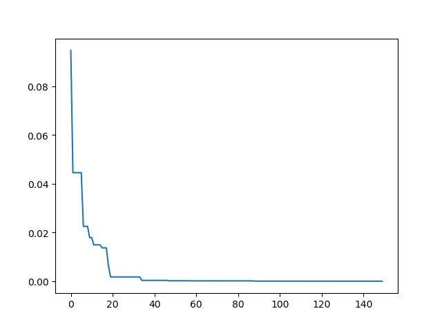
-> Demo code: examples/demo_pso.py#s4
pso = PSO(func=demo_func, dim=3)
fitness = pso.run()
print('best_x is ', pso.gbest_x, 'best_y is', pso.gbest_y)Step1: define your problem
-> Demo code: examples/demo_sa.py#s1
demo_func = lambda x: x[0] ** 2 + (x[1] - 0.05) ** 2 + x[2] ** 2Step2: do SA
-> Demo code: examples/demo_sa.py#s2
from sko.SA import SA

sa = SA(func=demo_func, x0=[1, 1, 1], T_max=1, T_min=1e-9, q=0.99, L=300, max_stay_counter=150)
best_x, best_y = sa.run()
print('best_x:', best_x, 'best_y', best_y)Step3: Plot the result
-> Demo code: examples/demo_sa.py#s3
import matplotlib.pyplot as plt
import pandas as pd

plt.plot(pd.DataFrame(sa.best_y_history).cummin(axis=0))
plt.show()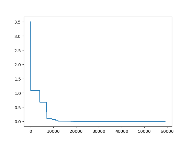
Step1: oh, yes, define your problems. To boring to copy this step.
Step2: DO SA for TSP
-> Demo code: examples/demo_sa_tsp.py#s2
from sko.SA import SA_TSP

sa_tsp = SA_TSP(func=cal_total_distance, x0=range(num_points), T_max=100, T_min=1, L=10 * num_points)

best_points, best_distance = sa_tsp.run()
print(best_points, best_distance, cal_total_distance(best_points))Step3: plot the result
-> Demo code: examples/demo_sa_tsp.py#s3
from matplotlib.ticker import FormatStrFormatter

fig, ax = plt.subplots(1, 2)

best_points_ = np.concatenate([best_points, [best_points[0]]])
best_points_coordinate = points_coordinate[best_points_, :]
ax[0].plot(sa_tsp.best_y_history)
ax[0].set_xlabel("Distance")
ax[0].set_ylabel("Iteration")
ax[1].plot(best_points_coordinate[:, 0], best_points_coordinate[:, 1],
           marker='o', markerfacecolor='b', color='c', linestyle='-')
ax[1].xaxis.set_major_formatter(FormatStrFormatter('%.3f'))
ax[1].yaxis.set_major_formatter(FormatStrFormatter('%.3f'))
ax[1].set_xlabel("Longitude")
ax[1].set_ylabel("Latitude")
plt.show()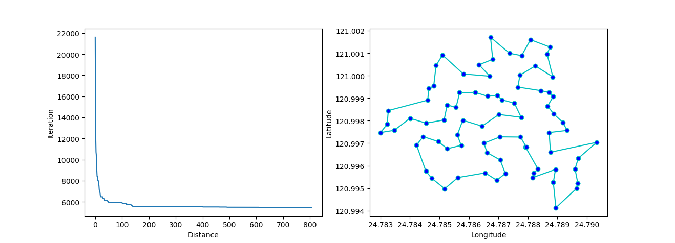
More: Plot the animation:
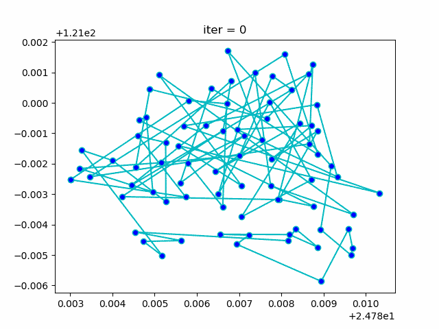
-> Demo code: examples/demo_aca_tsp.py#s2
from sko.ACA import ACA_TSP

aca = ACA_TSP(func=cal_total_distance, n_dim=8,
              size_pop=10, max_iter=20,
              distance_matrix=distance_matrix)

best_x, best_y = aca.run()
-> Demo code: examples/demo_ia.py#s2
from sko.IA import IA_TSP

ia_tsp = IA_TSP(func=cal_total_distance, n_dim=num_points, pop=500, max_iter=2000, Pm=0.2,
                T=0.7, alpha=0.95)
best_points, best_distance = ia_tsp.run()
print('best routine:', best_points, 'best_distance:', best_distance)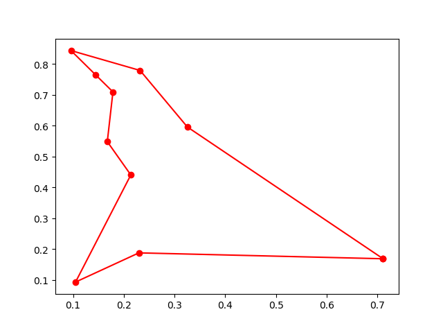
-> Demo code: examples/demo_asfs.py#s1
def func(x):
    x1, x2 = x
    return 1 / x1 ** 2 + x1 ** 2 + 1 / x2 ** 2 + x2 ** 2


from sko.ASFA import ASFA

asfa = ASFA(func, n_dim=2, size_pop=50, max_iter=300,
            max_try_num=100, step=0.5, visual=0.3,
            q=0.98, delta=0.5)
best_x, best_y = asfa.fit()
print(best_x, best_y)