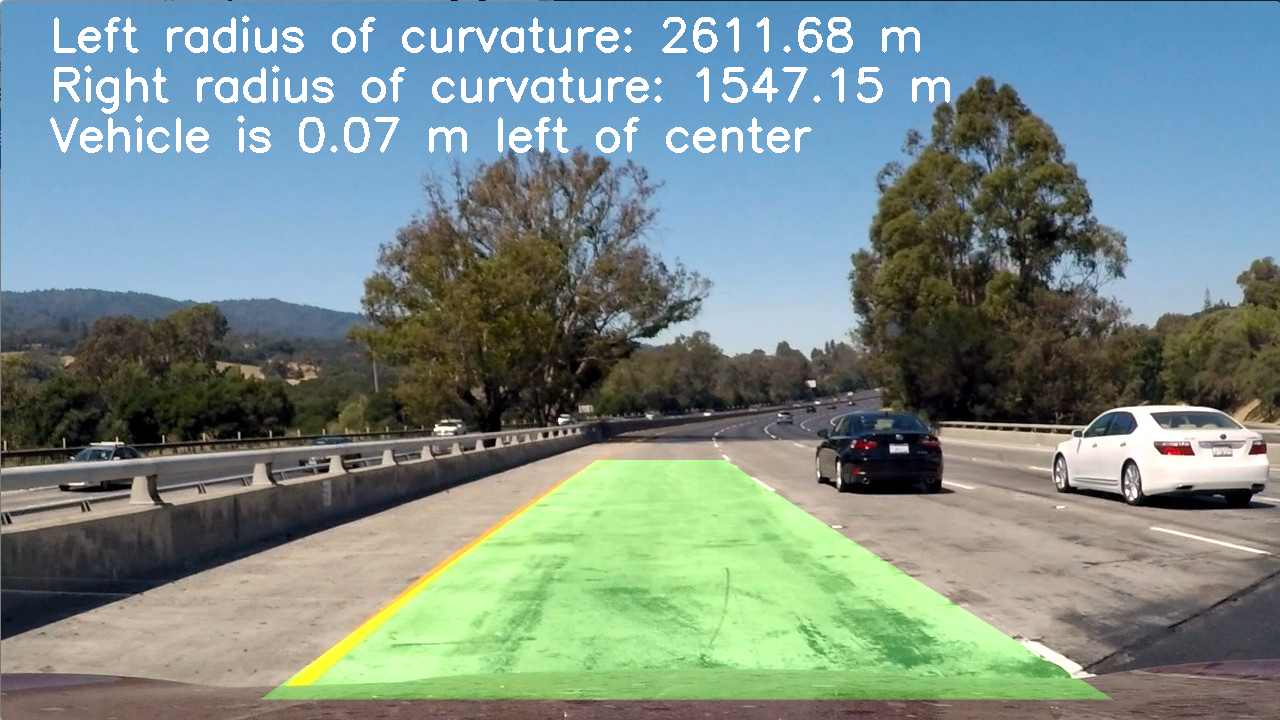
The objective of this project is to write a software pipeline to identify the lane boundaries in a video. The goals / steps are the following:
- Compute the camera calibration matrix and distortion coefficients given a set of chessboard images.
- Apply a distortion correction to raw images.
- Use color transforms, gradients, etc., to create a thresholded binary image.
- Apply a perspective transform to rectify binary image ("birds-eye view").
- Detect lane pixels and fit to find the lane boundary.
- Determine the curvature of the lane and vehicle position with respect to center.
- Warp the detected lane boundaries back onto the original image.
- Output visual display of the lane boundaries and numerical estimation of lane curvature and vehicle position.
The images for camera calibration are stored in the folder called camera_cal. The images in test_images are for testing your pipeline on single frames.
For details on implementation refer to this file.
Rubric Points
1. Briefly state how you computed the camera matrix and distortion coefficients. Provide an example of a distortion corrected calibration image.
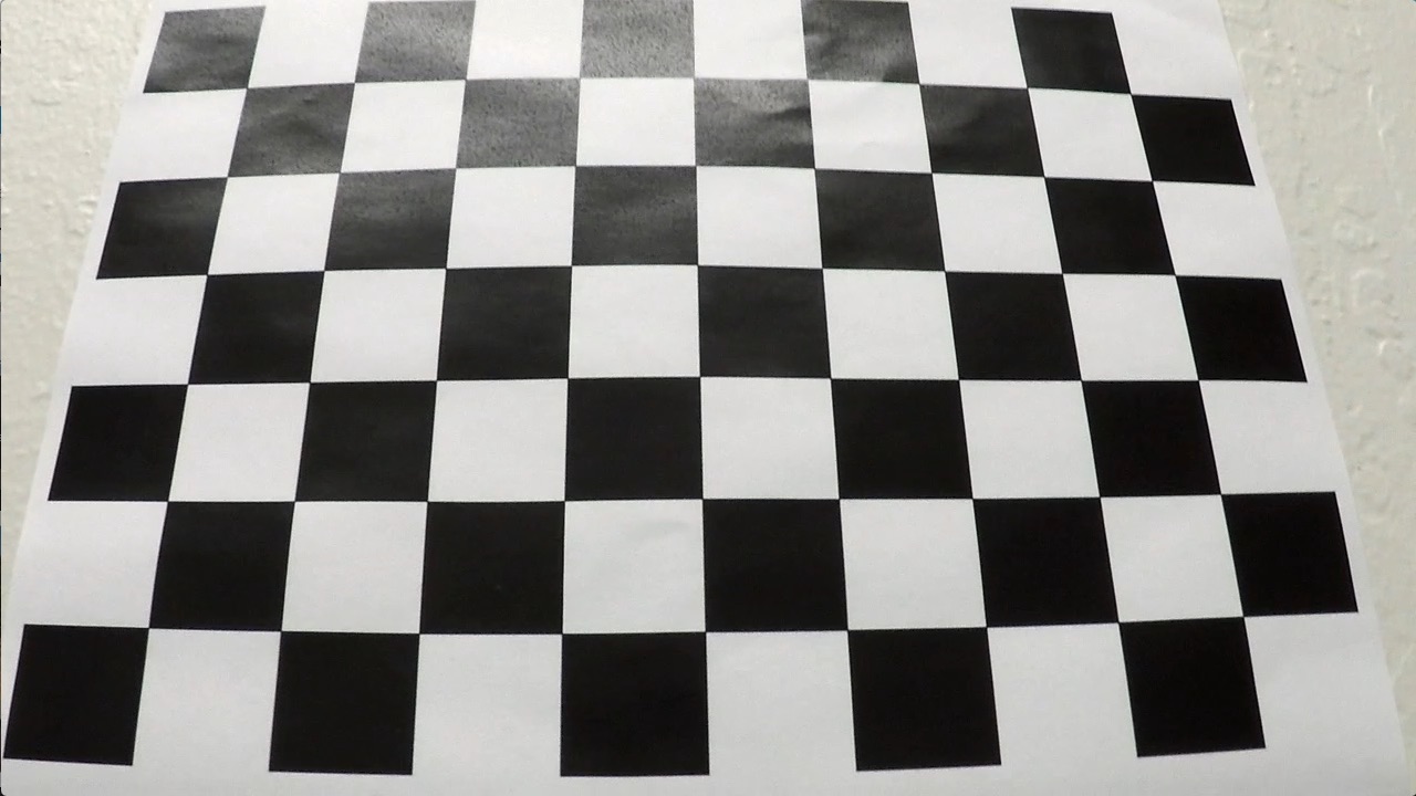
The first step for detecting lanes in an image is to perform camera calibration to identify the matrix and distortion coefficients that describe the camera. To achieve this, we need to map arbitrary points in a camera image to their corresponding points in an undistorted image. For this purpose, we leverage images of chessboards as mapping corners between original and corrected versions is relatively straight forward.
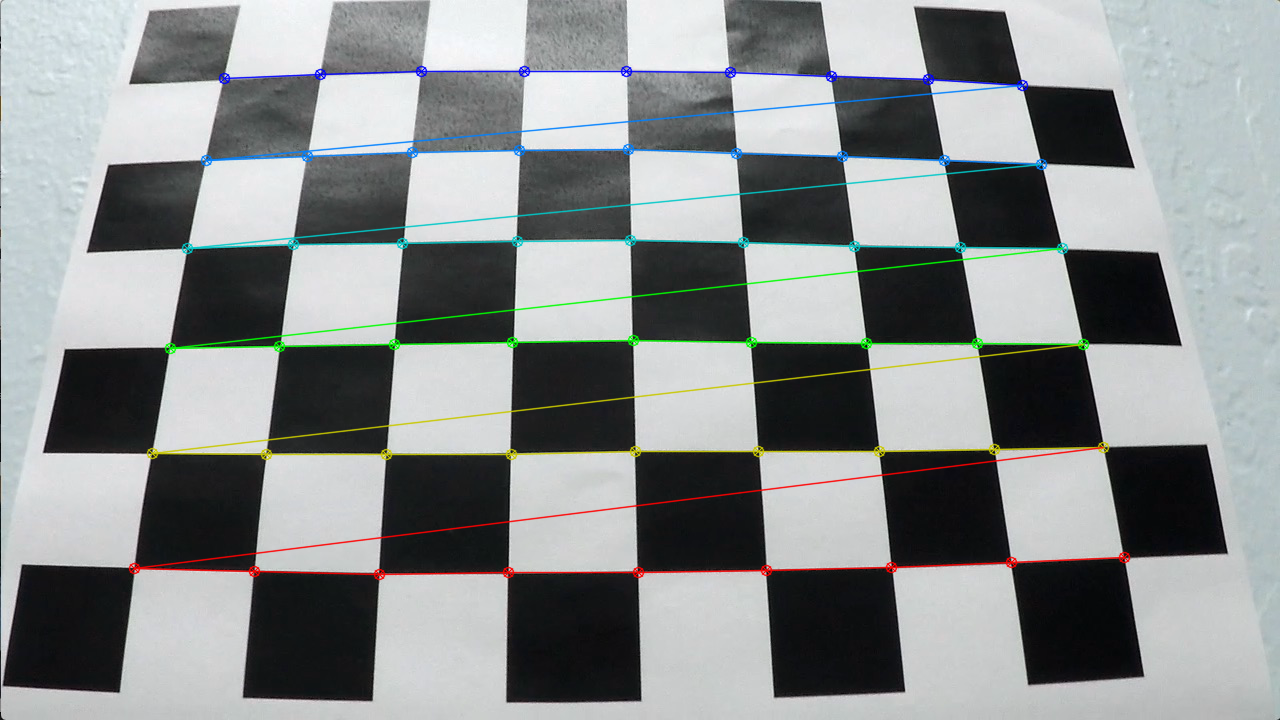
To begin, we prepare "object points", which refer to a 3-dimensional grid created to represent coordinates in the real world. The corrected chessboard image will be assummed to be fixed on the (x,y) plane at z=0, such that object points remain the same across images. Then, iterating through the available calibration images, we proceed to find cheesboard corners through the cv2.findChessboardCorners() function. Every time corners are found, the corners coordinates (x,y) will be appended to a list imgpoints and the object points to a list objpoints.
Once we have iterated through all images we proceed to compute the camera calibration and distortion cousing the cv2.calibrateCamera() function.
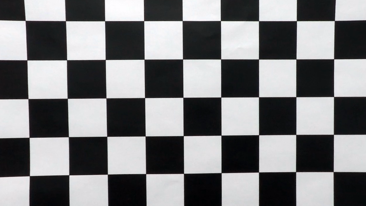
Then, we leverage the function cv2.undistort() to correct the image.
- Distortion Correction
- Tranformations To A Binary Image
- Perspective Transform
- Detect Line Boundaries
- Lane Curvature & Vehicle Center
- Unwarp Image
- Render Lane Lines
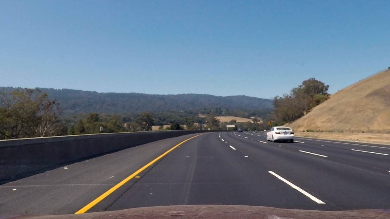
After the camera matrix and distortion coefficients are available, these can be leveraged to undistort any images taken from the same camera. Once again, to undistort the image, we can use the function cv2.undistort(). An example of an undistorted image can be seen below.
2. Describe how (and identify where in your code) you used color transforms, gradients or other methods to create a thresholded binary image. Provide an example of a binary image result.
The next step is to perform transformations on the undistorted image to will facilitate the recognition of lane lines. Suitable transformations include color adjustments, such as converting to gray scale or other color spaces, color thresholding, to filter our pixels within a color range, and gradient thresholding, to expose variations in color and light across the image.
The steps I followed for my project can be highlighted as follows:
Gradient Threshold
-
Convert the image to gray scale.
python cv2.cvtColor(img, cv2.COLOR_RGB2GRAY) -
Calculate the color gradient along the x and y axis.
    sobel_x = get_gradient(gray, True, sobel_kernel = 7)
    sobel_y = get_gradient(gray, False, sobel_kernel = 7)
The kernel refers to the amount of pixels we should leverage to calculate the gradient (i.e. 7 x 7)
- Preserve pixels with a gradient across the x-axis (vertical lines) between 20 and 220.
apply_gradient_thresholds(sobel_x, threshold = (20,220))This function will filter pixels within the range using the absolute gradient.
- Preserve pixels with a gradient direction between 40 and 70 degrees.
apply_direction_thresholds(sobel_x, sobel_y, threshold = (40*np.pi/180, 70*np.pi/180))This excludes almost horizontal or vertical lines. The formula to calculate the gradient is as follows:
np.arctan2(np.absolute(gradient_y), np.absolute(gradient_x))- Preserve pixels with a magnitude between 20 and 200
apply_gradient_thresholds(sobel_x, threshold = (20,220))The formula to calculate the magnitude of the gradient is as follows:
magnitude = np.sqrt(gradient_x**2 + gradient_y**2)Color Threshold
- With the image in RGB color space, preserve pixels with a Red channel between 210 and 255
apply_red_threshold(img, (210,255))This will preserve pixels closer to yellow and white on the red channel.
- With the image in HLS color space, preserve pixels with a Saturation channel between 90 and 255.
apply_saturation_threshold(img, (90, 255))Preserve mor colorful pixels.
Then, preserve pixels when either the gradient or color thresholds are met.
combined[(gradient_masks == 1) | (color_masks == 1)] = 1An example of the output of this process can be found below:
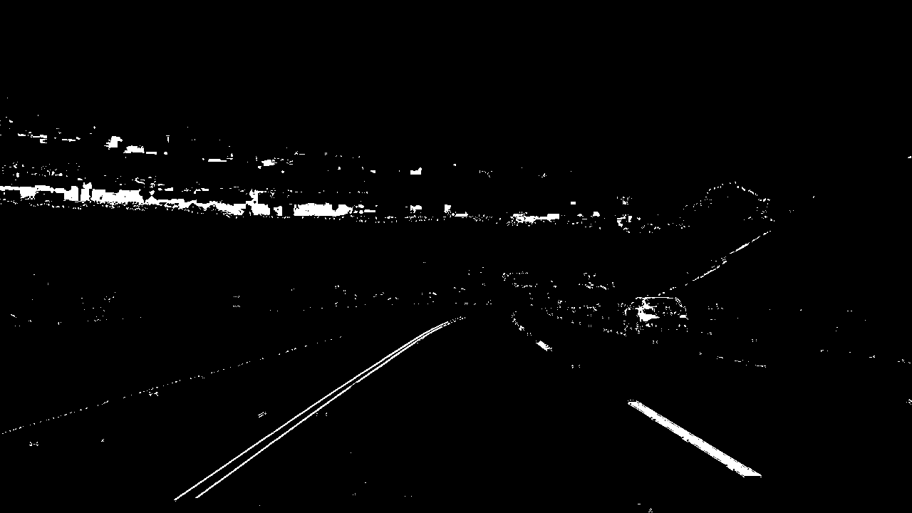
The section containing the implementation can be found on the Transformation to A Binary Image Section
3. Describe how (and identify where in your code) you performed a perspective transform and provide an example of a transformed image.
The next step is to transform the image into a bird's eye view perspective in order to see lanes from "above". Since lanes are parallel, it should help us to identify the exact pixels belonging to both the left and right lanes. To achieve this, we need to "map" points in the original image (src) into how they would look from above (dst), which would be essentially a rectangle.
The function below apply_perspective_transform() takes as inputs an image (img), as well as source (src) and destination (dst) points in order to provide the Matrix required to transform these points, and the inverse to convert them back to original space.
    def apply_perspective_transform(img, src, dst):

        img_size = (img.shape[1], img.shape[0])

        M = cv2.getPerspectiveTransform(src, dst)
        Minv = cv2.getPerspectiveTransform(dst, src)
        warped = cv2.warpPerspective(img, M, img_size, flags=cv2.INTER_LINEAR)

        return M, Minv, warped
For source and destination points I hardcoded them as follows:
    src = np.float32([[280,  700],  # Bottom left
                      [595,  460],  # Top left
                      [725,  460],  # Top right
                      [1125, 700]]) # Bottom right

    dst = np.float32([[width*.2,  height],  # Bottom left
                      [width*.2,  0],  # Top left
                      [width*.8,  0],  # Top right
                      [width*.8, height]]) # Bottom right
An exmaple of transforming a picture in bird's eye view can be seen below:
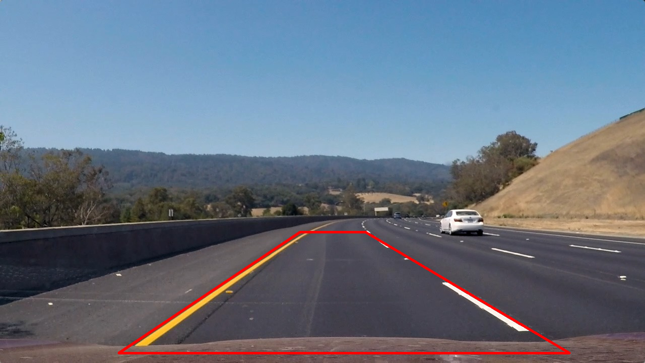
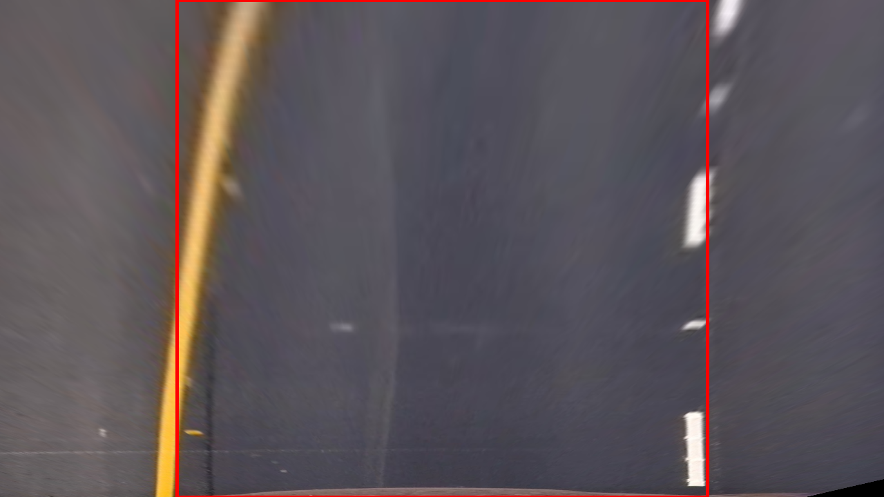
The section containing the implementation can be found on the Perspective Transform Section
4. Describe how (and identify where in your code) you identified lane-line pixels and fit their positions with a polynomial?
Next, we can proceed to identify lane-line pixels by identifying the areas with the most pixels remaining after thresholding in step 3. To start, we would naturally start at the beginning of the lane (closer to the bottom of the image). We can plot a histogram of the number of pixels ("activations") across the y-axis we find for every 1 pixel we move in the x-axis direction.
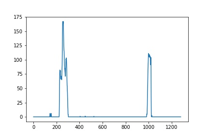
From there, we can start our search in the pixels that register the most "activations". We can split the height of the image in windows and designate a search margin within the pixels above to identify all "activated" pixels within the window. We can repeat this step for all subsequent windows, recalculating our center if too many pixels are found. Finally, once we have all our windows, we can fit a polinomial of second-degree across all the pixels we found within our windows to identify the lane.
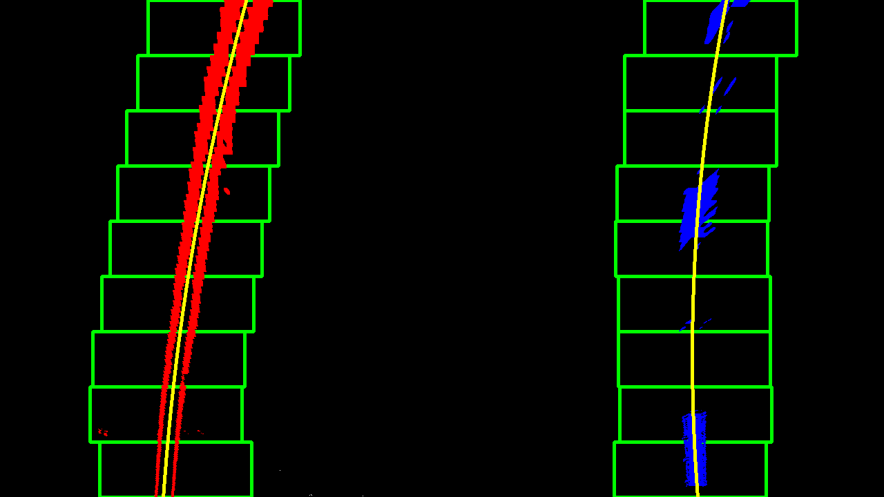
- Implementaion in function
detect_lane_lines*
However, it is true that lanes don't move that much between frames, so we could potentially use the polynomial of previous frames to guide our search. An example is as follows:
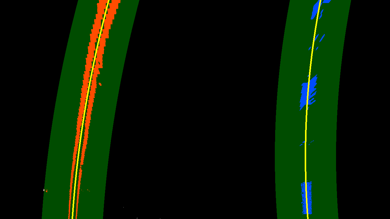
- Implementaion in function
detect_lane_lines_bias*
The section containing the implementation can be found on the Detecting Line Boundaries Section
5. Describe how (and identify where in your code) you calculated the radius of curvature of the lane and the position of the vehicle with respect to center.
The next step is to calculate the radius of the curvature of the lane and how far the vehicle is frmo the center so that we can provide that information in each frame.
The formula to calculate the radius of the curvature is found below, where A and B are the first two coefficients of a second degree polynomial fitted to the lane lines we found above.
curve_rad = ((1 + (2*A*y*ym_per_pix + B)**2)**1.5) / np.absolute(2*A)It must also be noted that we have to add conversion factors between pixels and meters to provide real measurements as opposed to image pixels. These should correspond with lane length and width in the real world.
| X - m to px | Y - m to px |
|---|---|
| 30/720 | 3.7/700 |
The section containing the implementation can be found on the Lane Curvature & Vehicle Center Section
6. Provide an example image of your result plotted back down onto the road such that the lane area is identified clearly.
Finally, we proceed to tranform the image back to the original perspective and overlay the lane we found onto the original image. To complete this step I created a highlight_lane functions that receives polynomials corresponding to the left and right lane and highlights the space in between them as green. An example of the final output can be seen below:
The section containing the implementation can be found on the Render Lane Lines
1. Provide a link to your final video output. Your pipeline should perform reasonably well on the entire project video (wobbly lines are ok but no catastrophic failures that would cause the car to drive off the road!).
Here's a link to my video result
1. Briefly discuss any problems / issues you faced in your implementation of this project. Where will your pipeline likely fail? What could you do to make it more robust?
While the video performance is favourable, the pipeline will likely fail under low light conditions such as shadows and heavily curved lanes. The reason for this is related to the manual thresholds identified that are not optimized for lanes and pictures under all possible conditions.
There are a number of potential improvements that can be implemented to improve performance of the pipeline. First, for thresholding images, different thresholds could be provided depending on the overall lightness of the image. That way, shadows or excessive sunlight in the image wouldn't interfere with line detection. Next, when identifying lane pixels, depending on the curvature of the lane and overall change between frames, parallel calculations could be triggered to validate findings with multiple pipelines.
However, these transformations are more suited for a machine learning solution using convolutional neural networks. That way, we can use the images to train our algorithm and allow it to select the most feasible thresholds and final function to determine what features of an image are more relevant to identify lane lines.

