This pipeline consists of 8 steps:
- Colour Selection
- Grayscale Conversion
- Gaussian Blur
- Edge Detection with Canny Transform
- Region of Interest Crop
- Hough Lines
- Line Combination
- Image Combination
Each step is described in the following, and an example is shown with the following image:
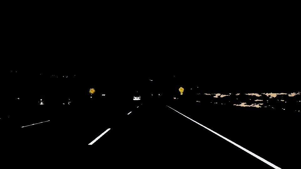
The first step is to select only the yellow and white pixels for lane detection. This is achieved in the following procedure using OpenCV functions:
- Set an upper and lower HLS threshold for the yellow and white colours
- Convert the image to HLS
- Filter the images using the thresholds to create an image with only yellow pixels and an image with only white pixels
- Combine the white and yellow images
- Use the combined image as a mask to select only the yellow and white pixels in the original RGB image.
HSL is used since this colour space makes it easier to isolate yellow and white from the rest of the image. The output of this step looks like this:
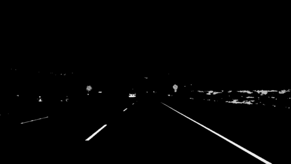
The next step is to do a grayscale conversion, which is done with a simple OpenCV conversion. This is done to simplify the further procedure as colour is no longer needed for edge detection. The output of this step looks like this:
Next, the Gaussian blur is performed to reduce the effects of noise, which will make edge detection much more difficult. This is also achieved with a simple OpenCV function. Different kernel sizes were experimented, and it is found that a size of 3 achieved the best results.The output of this step looks like this:
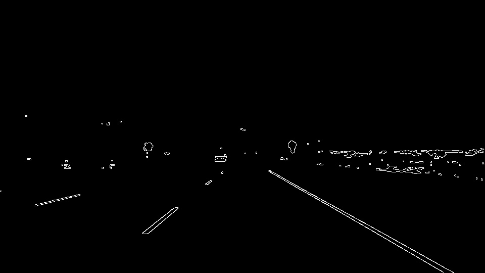
After, the Canny edge detection was accomplished with a simple OpenCV function. The Canny edge detection requires and upper and lower threshold as parameters, where the upper threshold sets the gradient limit for strong edges that will be included in the edge detection. Any gradient below the lower threshold is discarded as an edge, and gradients between the threshold will be included if it is connected to a strong edge. Recommended high:low thresholds rations are 3:1 or 2:1, and it was experimentally found that a lower threshold of 100 and a high threshold of 300 achieved good results. The output of the Canny edge detection is a black image with white pixels along the edges.The output of this step looks like this:
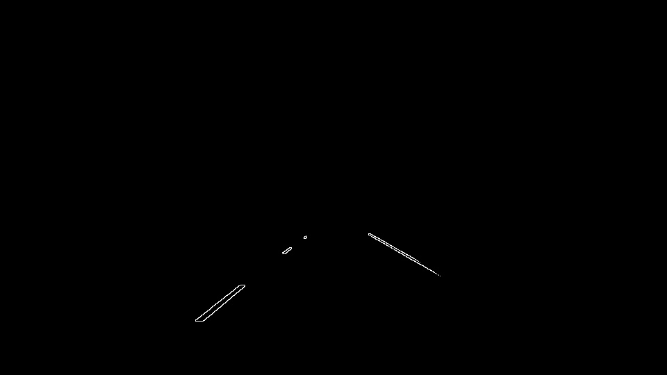
The edge detection algorithm outputs all edges in an image, but it is desired to only have the edges that correspond to lane lines. Therefore, a region of interest in image space can be defined where the lanes will occur inside. This can be formed using trapezoid connecting the bottom of the screen to about halfway up the screen with edges parallel to the lane lines. This will discard all edges from adjacent lanes, cars, etc.The output of this step looks like this:
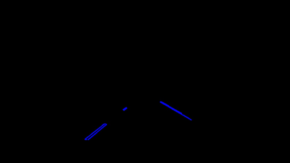
Next the edges need to have line segments fit through them. This is accomplished using a hough line transform, which looks at every point along the edge and finds the every possible line that fits through that point. These lines are plotted in hough space as polar coordinate parameters, and this is done for each point along the edge. The intersections in hough space correspond to lines that cross multiple points, which is likely to be a line segment that fits the edge. This is done using a voting system, and the output of this is multiple line segments along the edges.
The threshold for number of intersections to detect a line is set as 5, and the minimum number of points that can form a line is set as 5 as well. Lastly the maximum gap between two points to be considered in the same line is set as 2. The output of this step looks like this:
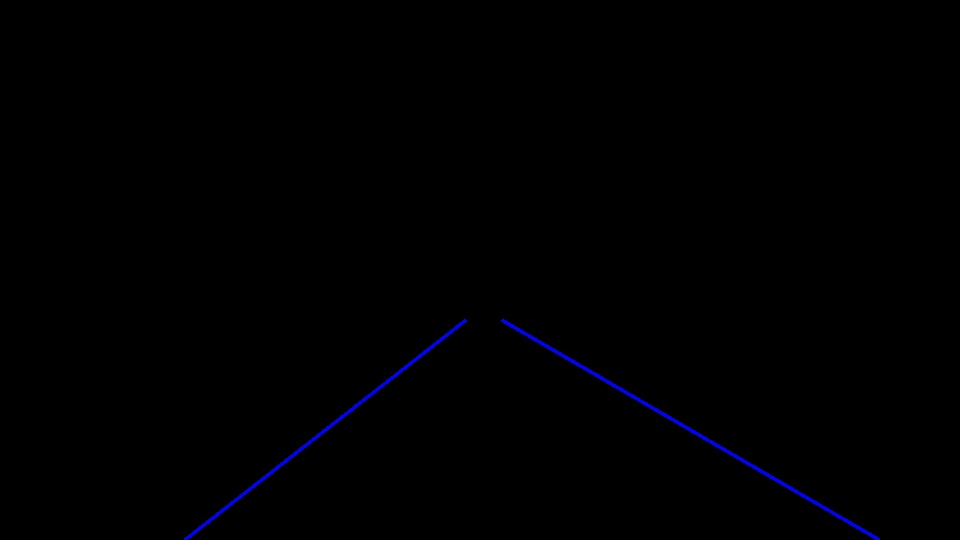
After getting line segments, these need to be combined to form one line for the left lane and one for the right. The first step is to classify each line using the slope. Slope values that are small are discarded (since they likely do not correspond to a lane), while negative slope values correspond to left lanes and positive slope values correspond to right lanes due to the coordinate system that OpenCV uses. Once classified, the start and end points of each line segment are used as points, and a least squares linear regression method is used to fit a line to the left points and the right points to create a line for the each lane. The output of this is an image with the two lanes drawn. The output of this step looks like this:
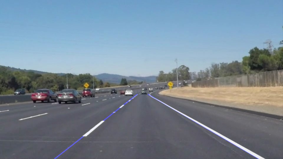
The original image and the image with the two lanes are combined using an OpenCV function using a weighting function. This produces the final image for the pipeline, which is shown here:
One potential shortcoming would be the inability to handle any non-straight roads. This pipeline assumes the lanes are straight, but curved or banked roads will break this pipeline since a straight line is fit to the data points during the Line Combination step.
Another short coming is the inability to handle outliers in the line fitting method, as using least-squares method is highly susceptible to outliers.
To address the short coming of curved roads, higher order polynomials can be fit to the data points that will follow the curve of the road.
Secondly, the use of RANSAC rather than using least-squares will be beneficial to fit a single line to all of the edges.

