This is an implementation of the Task2Vec method described in the paper Task2Vec: Task Embedding for Meta-Learning.
Task2Vec provides vectorial representations of learning tasks (datasets) which can be used to reason about the nature of those tasks and their relations. In particular, it provides a fixed-dimensional embedding of the task that is independent of details such as the number of classes and does not require any understanding of the class label semantics. The distance between embeddings matches our intuition about semantic and taxonomic relations between different visual tasks (e.g., tasks based on classifying different types of plants are similar). The resulting vector can be used to represent a dataset in meta-learning applicatins, and allows for example to select the best feature extractor for a task without an expensive brute force search.
To compute and embedding using task2vec, you just need to provide a dataset and a probe network, for example:
from task2vec import Task2Vec
from models import get_model
from datasets import get_dataset

dataset = get_dataset('cifar10')
probe_network = get_model('resnet34', pretrained=True, num_classes=10)
embedding =  Task2Vec(probe_network).embed(dataset)
Task2Vec uses the diagonal of the Fisher Information Matrix to compute an embedding of the task. In this implementation
we provide two methods, montecarlo and variational. The first is the fastest and is the default, but variational
may be more robust in some situations (in particular it is the one used in the paper). You can try it using:
task2vec.embed(dataset, probe_network, method='variational')Now, let's try computing several embedding and plot the distance matrix between the tasks:
from task2vec import Task2Vec
from models import get_model
import datasets
import task_similarity

dataset_names = ('mnist', 'cifar10', 'cifar100', 'letters', 'kmnist')
dataset_list = [datasets.__dict__[name]('./data')[0] for name in dataset_names]

embeddings = []
for name, dataset in zip(dataset_names, dataset_list):
    print(f"Embedding {name}")
    probe_network = get_model('resnet34', pretrained=True, num_classes=int(max(dataset.targets)+1)).cuda()
    embeddings.append( Task2Vec(probe_network, max_samples=1000, skip_layers=6).embed(dataset) )
task_similarity.plot_distance_matrix(embeddings, dataset_names)
You can also look at the notebook small_datasets_example.ipynb for a runnable implementation of this code snippet.
First, decide where you will store all the data. For example:
export DATA_ROOT=./data
To download CUB-200, from the repository root run:
./scripts/download_cub.sh $DATA_ROOTTo download iNaturalist 2018, from the repository root run:
./scripts/download_inat2018.sh $DATA_ROOTWARNING: iNaturalist needs ~319Gb for download and extraction. Consider downloading and extracting it manually following the instructions here.
To compute the embedding on a single task of CUB + iNat2018, run:
python main.py task2vec.method=montecarlo dataset.root=$DATA_ROOT dataset.name=cub_inat2018 dataset.task_id=$TASK_ID -mThis will use the montecarlo Fisher approximation to compute the embedding of the task number $TASK_ID in the CUB + iNAT2018 meta-task.
The result is stored in a pickle file inside outputs.
To compute all embeddings at once, we can use Hydra's multi-run mode as follow:
python main.py task2vec.method=montecarlo dataset.root=$DATA_ROOT dataset.name=cub_inat2018 dataset.task_id=`seq -s , 0 50` -mThis will compute the embeddings of the first 50 tasks in the CUB + iNat2018 meta-task.
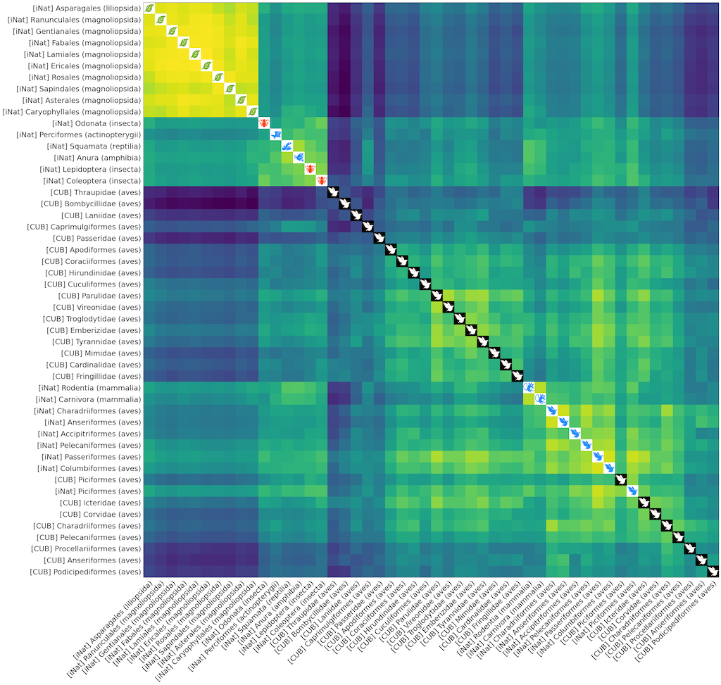
To plot the 50x50 distance matrix between these tasks, first download all the iconic_taxa
image files
to ./static/iconic_taxa, and then run:
python plot_distance_cub_inat.py --data-root $DATA_ROOT ./multirun/montecarloThe result should look like the following. Note that task regarding classification of similar life forms (e.g, different types of birds, plants, mammals) cluster together.
