This is a work-in-progress.
This repository contains the GNU Radio flowgraphs for the GRCon 2020 lightning talk 'Seeing Signals: Real-Time Visualization of A Delay-and-Sum Beamformer'. The flowgraph simulations and demonstrations show how 2D visualization of magnitudes and direction of arrival can be generated from phased arrays using a delay-and-sum beamformer. By using raster plots it’s possible to view both direction of arrival and magnitude for all steering weights simultaneously. This is a simple approach to recieve-only beamforming.
I suggest that you start with the simulations. They should work in GNU Radio >= 3.8.2 and the main (3.9) branch. If you are using 3.8.1 or earlier, there's a bug with QT message ports so the simulations won't run (you'll see an error in the QT range blocks). Please do consider updating GNU Radio if that's the case. If you're on a Mac, the Video SDL Sink does not work properly. You can get around this by disabling the blocks.
The grcon folder includes the presentation slides, flowgraph simulations, flowgraphs for demos with USRP B210s, and screen captures of the flowgraphs.
The best way to try this out is to run the simulations, starting with the 1 dimension demo. There is a simulated transmitter that can move a signal back and forth.
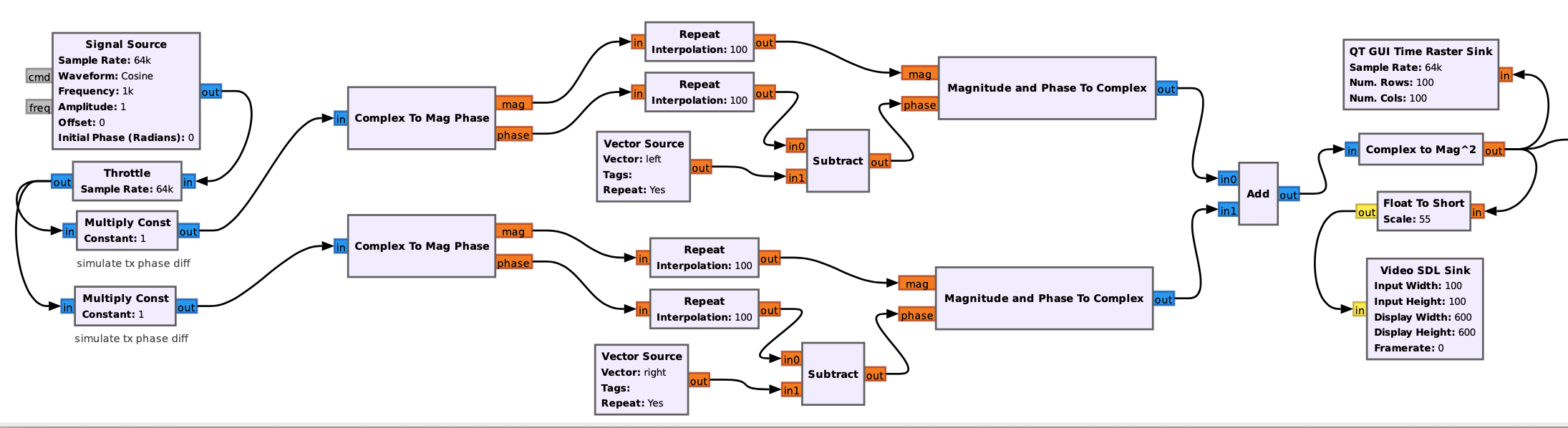
The complex signals are converted to magnitude and phase. The signals are repeated 100 times. This var in the flowgraph, columns is the number of pixels in the heatmap. The phase lag is added. These are pairs. When one signal is lagged by some radians, the other is lagged 0. The signals are converted back to complex again, and then added. The magnitude-squared is now the pixel value.
The phase lags (steering vector or weights) are created in the variable blocks. Here's the annotated code in Python (copied from the flowgraph):
import numpy as np # use the import block

maxtheta = 150 # beam width of the phased array
columns = 100 # number of pixels for the heatmap
# create linearly spaced values for one half the columns, between 0 and beamwidth, but not including 0.
shiftarrL = np.radians(np.linspace(start=maxtheta, stop=0, num=int(columns/2), endpoint=False))
# pad out the rest of the columns with 0s, only one stream can be lagged in 1d
left = np.pad(shiftarrL, (0, int(columns/2)), 'constant')
# don't do it all again, just flip the left to make the right
right = np.flip(left, axis=0)
# profit
print(left)
print(right)These flowgraphs can heavily interpolate. In one dimension, the demo interpolates by 100. In two dimensions, the simulation interpolates by 10,000 (100x100). Interpolating by 4 orders of magnitude can ruin your day if your beginning sample rate is high. This is why in the demos there is a Keep 1 in N block. Keep it in mind if you want to adapt to your own context. The Video SDL Sink is not very forgiving when being pushed by millions of samples.
In the highly unlikely event that this helps you towards scientific publication, I’d appreciate a citation:
Stanley, Richard. (2020) Seeing Signals: Real-time Visualization of a Delay-and-Sum Beamformer [Lightning Talk]. GRCon (GNU Radio Conference). Virtual. URL: https://github.com/citizenrich/seeingsignals