Pattern Recognition: Linear Regression

UVic Robotics Master. Perception.

Instructions

Clone this repository and write code to complete the assignments. When executed, your code must print the answers to the questions in each section, alongside the results that led to these conclusions. Module textwrap can be used to format long paragraphs of text and make them look nicer. An IPython notebook is an acceptable alternative to a plain Python program.

This is a personal assignment, please complete it individually.

Preliminaries

This and the next three homework assignments have to be completed using Python. Python is a very easy to learn and flexible programming language, with many libraries for the most diverse tasks.

For the homework in this course, we will use the following libraries, mostly from the SciPy family:

SciPy is a collection of libraries for scientific computing in Python.
Numpy provides the backbone functionality for numerical processing.
Matplotlib is a powerful plotting library.
Scikit Learn Is a simple and complete machine learning library for Python.
OpenCV is the reference computer vision and image processing library, with comprehensive Python bindings.

Besides these libraries, IPython is recommended as an extended and more friendly interactive Python interpreter. It is also necessary in order to view the course notebooks.

In Ubuntu, all the required software can be installed with the following commands:

$ sudo apt-get install python-scipy python-numpy python-matplotlib \
  python-opencv python-sklearn
$ sudo apt-get install ipython-notebook

Learning Python is extraordinarily easy, especially if other programming languages are already known. There are some tutorials to get up to speed in a few minutes:

Learn Python in 10 minutes tutorial for beginners
A very concise and recommendable Python+Numpy tutorial by Justin Johnson. Here the ipython notebook version
Official Python tutorial
OpenCV-Python tutorials

For this assignment, it is recommended to read at least the Python+Numpy tutorial.

Linear Regression

See the ipython notebook from the class for reference.

Q1) Get the Housing Data Set form the repository [Names, Data] (it is different from the one used in the notebook!).
Q2) Load the data (using numpy.loadtxt) and separate the last column (target value, MEDV). Compute the average of the target value and the MSE obtained using it as a constant prediction.
Q3) Split the data in two parts (50%-50%) for training and testing (first half for training, second half for testing). Train a linear regressor model for each variable individually (plus a bias term) and compute the MSE on the training and the testing set. Which variable is the most informative? which one makes the model generalize better? and worse? Compute the coefficient of determination (R^2) for the test set.

Hint: If you want to select the i-th column of an array, but want it to retain the two dimension, you can do it like that:
column = data_array[:,i:i+1] 

Q4) Now train a model with all the variables plus a bias term. What is the performance in the test set? Try removing the worst-performing variable you found in step 3, and run again the experiment. What happened?
Q5) We can give more capacity to a linear regression model by using basis functions (Bishop, sec. 3.1). In short, we can apply non-linear transformations to the input variables to extend the feature vector. Here we will try a polynomial function:

Repeat step 3 but adding, one by one, all polynomials up to degree 4. What are the effects of adding more capacity to the model?

Gradient Descent

As we have seen, overfitting is a problem that arises when we try to have more powerful methods, able to better adapt to the data. In order to reduce overfitting, we can regularize our model, but then we do not have a closed form solution and must resort to optimization. First we will use Gradient Descent, which is a widely used optimization algorithm. Here is a simple implementation in pseudo-code:

0. Function Gradient_Descent
1.   Initialize theta(0) at random
2.   t=0, maxit=100, step=1e-6, loss=zeros(maxit)
3.   loss(0) = f(theta)
4.   do
5.      t=t+1
6.      theta(t) = theta(t-1) - step * f'(theta(t-1))
7.      loss(t) = f(theta)
8.   While t<maxit
9.   return theta

Q6) The objective function f for Regularized Linear Regression is the following:

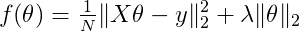
And its derivative f' is:

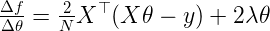
Implement two functions in Python, one that computes f and another that computes f'. As an optional exercise, work the derivation of the objective function.
Q7) Implement code to train a regularized linear regression model using gradient descent according to the previous pseudocode. Use it to train a model with all variables and then evaluate it in the test data.

This may be a difficult exercise. Here are some hints to help you finish it successfully:

lambda is a reserved word for nameless functions in Python; use a different name for the variable.

Make sure your f and f' functions are correct. Here are some values for reference:
f(data_train_with_bias, labels_train, theta_all_zeros, Lambda=1) = 660.1083
f'(data_train_with_bias, labels_train, theta_all_zeros, Lambda=1) = [ -48.62, -20.40, -676.58, -422.27, -3.90, -24.70, -317.49, -3033.81, -206.06, -222.99, -15327.84, -857.69, -18476.12, -477.47]
f(data_train_with_bias, labels_train, theta_all_0.01, Lambda=1) = 328.66 f'(data_train_with_bias, labels_train, theta_all_0.01, Lambda=1) = [ -31.98, -12.23, -485.03, -260.24, -2.55, -15.98, -212.42, -1923.15, -137.89, -146.50, -9899.61, -560.03, -12199.25, -285.86]

Start with only a few iterations, and check that your loss (computed with f ) is decreassing. If it is increasing or doing a zig-zag, lower your learning step.

To start, use lambda=10 and step=1e-6.

Q8) Writting a good optimization routine is very difficult, with many particular choices and obscure techniques that require a vast knowledge of the field. Furthermore, except if you are doing research on the subject, in general it is not necessary to write your own function optimization code: there are many libraries that provide robust implementations. For the rest of the homework we will use fmin_l_bfgs_b as our optimizer. Read the online documentation to figure out how to use it, and train a model for our data.

Hint: You only need to worry about the first four parameters.

Model Selection

Q9) Different lambda values lead to different models, and we want to find the one that gives better results in new data. Unfortunately we cannot use the test data for this, since then we would have nowhere to test our final model. Instead, we will use cross-validation. In particular, you have to implement k-fold cross-validation. Next, use it to select the lambda parameter for a regularized linear regression model with fmin_l_bfgs_b as the optimizer. As data, use the polynomial expansion up to degree 5 of the LSTAT variable (last input variable). Using matplotlib, plot the evolution of the training and validation MSE as you increase the lambda parameter. Finally, print the MSE of the selected model in the test set.

Use the lambda values generated by the following expression:
 lambdas = [10**i for i in range(-6,7)]  
Pylab offers a very convenient interface to matplotlib. Here is a short example code:
 import pylab
 pylab.plot([1,2,3,4], [4,6,3,7], '-b')
 pylab.plot([1,2,3,4], [1,2,7,9], '-.r')
 pylab.title('Demo plot')
 pylab.legend(['first function', 'second function'])
 pylab.show()
You will want to use a logarithmic scale for the lambdas. To use it, just type:
 pylab.xscale('log') # or alternatively pylab.yscale('log')

Q10) We are almost done! In this last task we will visualize the effect of regularization in a cost surface. Using bias and a single variable our model has two parameters, which means we can plot each possible model in an area, and assign it a color based on the loss for the particular choice of parameters. Complete the following code, and use it to visualize the cost surface of the second variable (ZN) for several choices of lambda, ranging from very small to very large. As an optional exercise try alternating between the L2 norm to the L1 norm in the objective function. Describe what you observe.

def plot_cost_surface(f, features, labels, Lambda):
   from matplotlib import pyplot
   XX, YY = np.meshgrid(np.arange(-10,10,0.1), np.arange(-10,10,0.1))
   ZZ = np.zeros(XX.shape)
   for i in range(XX.shape[0]):
       for j in range(XX.shape[1]):
       #<COMPLETE THIS CODE>
   pyplot.imshow(ZZ)
   N=ZZ.shape[0]
   pyplot.title('Lambda = %.4f'%Lambda)
   pyplot.xticks([0,N/4,N/2,3*N/4,N-1],['-10','-5','0','5','10'])
   pyplot.yticks([0,N/4,N/2,3*N/4,N-1],['10','5','0','-5','-10'])
   pyplot.colorbar()
   pyplot.show()

Extra

In case you have not had enough, here are a couple of things you can try next:

The UCI repository has many datasets for regression collected over the years. Select one or a few, and try to solve them using the tools you have developed during this homework.
Think of how you would use linear regression to improve or automate some aspect of your work or daily life (doesn't need to make a lot of sense), and describe the way in which you would approach the problem.

chuski92 / RoboticaUVic-LinearRegression