This goal of this repo is to provide a gentle introduction to numerical methods for Bayesian inference. Papers on the topic are usually quite abstract and general, and existing implementations are too complex to be back engineered.
Here, you'll find different numerical solutions to a single, simple model: the logistic regression (see below). The various algorithms are voluntarily reduced to their bare minimum in order to provide simple working examples. Hopefully, this code will provide some insight into the different approaches, their strengths, and theirs limitations.
Imagine a simple psychophysic experiment in which we present the subject with a sequence stimuli of various intensities. The probability of the subject detecting the stimulus increases with its intensity:
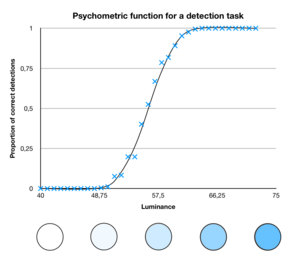
Let's denote x the stimulus intensity. If we assume that the task is calibrated such that the subject is at chance level for a neutral simulus (x = 0), we can write the psychometric function that maps the stimulus intensity to the probability of detection using a sigmoid function:
where theta is a parameter that capture the sensitivity of the subject to changes in intensities. This function is implemented in sigmoid.m.
At each trial, the subject can only give a binary answer (y), "seen" (y = 1) or "not seen" (y = 0). Formally, we can describe the probability distribution of the responses, aka. the Likelihood function, as a Bernoulli distribution, ie:
The function simulate_data(true_theta) will simulate 100 artificial responses for a sequence of stimuli between -5 and 5 for a given sensitivity parameter true_theta.
Our goal is to perform Bayesian inference to invert the logistic model.
The function [posterior, logEvidence] = main() will generate artificial data, define a prior, and run a set of inversion routines that will approximate both the posterior and the (log-)model evidence. More precisely, it will implement:
- An MCMC scheme: the Metropolis-Hastings algorithm, with a rough approximation of the model evidence via the Harmonic estimator (
invert_monte_carlo.m). - A Variational-Laplace scheme, as implemented in SPM or the VBA toolbox (
invert_variational_laplace) - A Variational procedure without Laplace. Although this method is never used in practice, it can help dissociate the influence of the Gaussian approximation of the posterior from the Laplace approximation (
invert_variational_numeric). - A Stochastic Gradient "blackbox" scheme (
invert_variational_stochastic), as usually found in machine learning - An easy inversion using the VBA-toolbox (
invert_VBAtoolbox)
- Murphy, K. P. (2007). Conjugate Bayesian analysis of the Gaussian distribution.
- Zhang, C., Butepage, J., Kjellstrom, H., & Mandt, S. (2018). Advances in variational inference. IEEE transactions on pattern analysis and machine intelligence.
- Daunizeau, J. (2017). The variational Laplace approach to approximate Bayesian inference. arXiv preprint arXiv:1703.02089.
- Friston, K., Mattout, J., Trujillo-Barreto, N., Ashburner, J., & Penny, W. (2007). Variational free energy and the Laplace approximation. Neuroimage, 34(1), 220-234.
- Ranganath, R., Gerrish, S., & Blei, D. (2014, April). Black box variational inference. In Artificial Intelligence and Statistics (pp. 814-822).
- Neal, R. M. (1993). Probabilistic inference using Markov chain Monte Carlo methods (pp. 93-1). Toronto, Ontario, Canada: Department of Computer Science, University of Toronto.
- Geyer, C. J. (2011). Introduction to markov chain monte carlo. Handbook of markov chain monte carlo, 20116022, 45.
- Andrieu, C., De Freitas, N., Doucet, A., & Jordan, M. I. (2003). An introduction to MCMC for machine learning. Machine learning, 50(1-2), 5-43.
- Friel, N., & Wyse, J. (2012). Estimating the evidence–a review. Statistica Neerlandica, 66(3), 288-308.
- Stephan, K. E., Penny, W. D., Daunizeau, J., Moran, R. J., & Friston, K. J. (2009). Bayesian model selection for group studies. Neuroimage, 46(4), 1004-1017.
- Rigoux, L., Stephan, K. E., Friston, K. J., & Daunizeau, J. (2014). Bayesian model selection for group studies—revisited. Neuroimage, 84, 971-985.
- Penny, W. D., Stephan, K. E., Daunizeau, J., Rosa, M. J., Friston, K. J., Schofield, T. M., & Leff, A. P. (2010). Comparing families of dynamic causal models. PLoS computational biology, 6(3), e1000709.
- Piray, P., Dezfouli, A., Heskes, T., Frank, M. J., & Daw, N. D. (2019). Hierarchical Bayesian inference for concurrent model fitting and comparison for group studies. PLoS computational biology, 15(6), e1007043.