This is an R Markdown document. Markdown is a simple formatting syntax for authoring HTML, PDF, and MS Word documents. For more details on using R Markdown see http://rmarkdown.rstudio.com.
When you click the Knit button a document will be generated that includes both content as well as the output of any embedded R code chunks within the document. You can embed an R code chunk like this: #Load Packages
if(!require("pacman")) install.packages("pacman")## Loading required package: pacman
pacman::p_load(forecast, tidyverse, gplots, GGally, mosaic,
               scales, mosaic, mapproj, mlbench, data.table,ggplot2, ggpubr)
#Reading the Utilities File
getwd()## [1] "C:/Users/chitr/OneDrive - The University of Texas at Dallas/Masters Collection/1st Sem/BA with R/HW1"
utilities <- read.csv("Utilities.csv")
str(utilities)
## 'data.frame': 22 obs. of 9 variables:
## $ Company : chr "Arizona " "Boston " "Central " "Commonwealth" ...
## $ Fixed_charge : num 1.06 0.89 1.43 1.02 1.49 1.32 1.22 1.1 1.34 1.12 ...
## $ RoR : num 9.2 10.3 15.4 11.2 8.8 13.5 12.2 9.2 13 12.4 ...
## $ Cost : int 151 202 113 168 192 111 175 245 168 197 ...
## $ Load_factor : num 54.4 57.9 53 56 51.2 60 67.6 57 60.4 53 ...
## $ Demand_growth: num 1.6 2.2 3.4 0.3 1 -2.2 2.2 3.3 7.2 2.7 ...
## $ Sales : int 9077 5088 9212 6423 3300 11127 7642 13082 8406 6455 ...
## $ Nuclear : num 0 25.3 0 34.3 15.6 22.5 0 0 0 39.2 ...
## $ Fuel_Cost : num 0.628 1.555 1.058 0.7 2.044 ...
##Creating DataTable
library(data.table)
Utilities_dt <- setDT(utilities)
##Creating the summary
Utilities_dt[,sapply(.SD, summary), .SDcols=names(Utilities_dt)[-1]]## Fixed_charge RoR Cost Load_factor Demand_growth Sales
## Min. 0.750000 6.40000 96.0000 49.80000 -2.200000 3300.000
## 1st Qu. 1.042500 9.20000 148.5000 53.77500 1.450000 6458.250
## Median 1.110000 11.05000 170.5000 56.35000 3.000000 8024.000
## Mean 1.114091 10.73636 168.1818 56.97727 3.240909 8914.045
## 3rd Qu. 1.190000 12.35000 195.7500 60.30000 5.350000 10128.250
## Max. 1.490000 15.40000 252.0000 67.60000 9.200000 17441.000
## Nuclear Fuel_Cost
## Min. 0.0 0.309000
## 1st Qu. 0.0 0.630000
## Median 0.0 0.960000
## Mean 12.0 1.102727
## 3rd Qu. 24.6 1.516250
## Max. 50.2 2.116000
##Calculating the standard Deviation
Utilities_dt[,sapply(.SD, sd), .SDcols=names(Utilities_dt)[-1]]## Fixed_charge RoR Cost Load_factor Demand_growth
## 0.1845112 2.2440494 41.1913495 4.4611478 3.1182503
## Sales Nuclear Fuel_Cost
## 3549.9840305 16.7919198 0.5560981
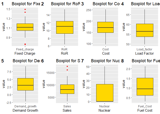
###Difference in Median and mean of percent nuclear are large so the distribution will be skewed.We are getting few outliers in Fixed_charge and Sales as we can see from mean and quartile range when compared with min and max values of the variables.Sales is comparatively larger in terms of variability over other variables since the standard deviation of sales is the largest ## Including Plots
Melted_FixedCharge <- melt(data = Utilities_dt, id.vars ="Company", measure.vars ="Fixed_charge")

Melted_RoR <- melt(data = Utilities_dt, id.vars ="Company", measure.vars ="RoR")
Melted_Cost <- melt(data = Utilities_dt, id.vars ="Company", measure.vars ="Cost")

Melted_LoadFactor <- melt(data = Utilities_dt, id.vars ="Company", measure.vars ="Load_factor")

Melted_DemandGrowth <- melt(data = Utilities_dt, id.vars ="Company", measure.vars ="Demand_growth")

Melted_Sales <- melt(data = Utilities_dt, id.vars ="Company", measure.vars ="Sales")

Melted_Nuclear <- melt(data = Utilities_dt, id.vars ="Company", measure.vars ="Nuclear")

Melted_FuelCost <- melt(data = Utilities_dt, id.vars ="Company", measure.vars ="Fuel_Cost")

BPFCharge <- ggplot(Melted_FixedCharge) +
  geom_boxplot(aes(x = variable, y = value),
               fill = "gold1", outlier.color = "firebrick2") +
  xlab("Fixed Charge") + ggtitle("Boxplot for Fixed Charge")

BPRoR <- ggplot(Melted_RoR) +
  geom_boxplot(aes(x = variable, y = value),
               fill = "gold1", outlier.color = "firebrick2") +
  xlab("RoR") + ggtitle("Boxplot for RoR")

BPMC <- ggplot(Melted_Cost) +
  geom_boxplot(aes(x = variable, y = value),
               fill = "gold1", outlier.color = "firebrick2") +
  xlab(" Cost") + ggtitle("Boxplot for Cost")

BPLF <- ggplot(Melted_LoadFactor) +
  geom_boxplot(aes(x = variable, y = value),
               fill = "gold1", outlier.color = "firebrick2") +
  xlab("Load Factor") + ggtitle("Boxplot for Load Factor")

BPDG <- ggplot(Melted_DemandGrowth) +
  geom_boxplot(aes(x = variable, y = value),
               fill = "gold1", outlier.color = "firebrick2") +
  xlab("Demand Growth") + ggtitle("Boxplot for Demand Growth")

BPMS <- ggplot(Melted_Sales) +
  geom_boxplot(aes(x = variable, y = value),
               fill = "gold1", outlier.color = "firebrick2") +
  xlab("Sales") + ggtitle("Boxplot for Sales")

BPMN <- ggplot(Melted_Nuclear) +
  geom_boxplot(aes(x = variable, y = value),
               fill = "gold1", outlier.color = "firebrick2") +
  xlab("Nuclear") + ggtitle("Boxplot for Nuclear")

BPFCost <- ggplot(Melted_FuelCost) +
  geom_boxplot(aes(x = variable, y = value),
               fill = "gold1", outlier.color = "firebrick2") +
  xlab("Fuel Cost") + ggtitle("Boxplot for Fuel Cost")

layout <- ggarrange(BPFCharge, BPRoR, BPMC, BPLF, BPDG, BPMS, BPMN, BPFCost,
                    labels = c("1", "2", "3", "4", "5", "6", "7", "8"), ncol = 4, nrow = 2)
layout
###Are there any extreme values for any of the variables ?Which ones?Explain your answers. ###There are two variables which are having extreme values or outliers as shown in the box plot.Fixed Charge and Sales.For fixed charge the range will be roughly from 0.96 to 1.26 ,there are 3 values less than 0.96 (i.e. Boston,Nevada,San Diego) and 4 variables above 1.26 range (i.e. Central,NY,Florida,Kentucky). ###For Sales there is 1 value less than lower limit (i.e. NY) and 4 values above the upper limit (i.e. Texas,Puget,Nevada,Idaho) ##Heat Map
library(reshape)##
## Attaching package: 'reshape'
## The following object is masked from 'package:data.table':
##
## melt
## The following object is masked from 'package:Matrix':
##
## expand
## The following object is masked from 'package:dplyr':
##
## rename
## The following objects are masked from 'package:tidyr':
##
## expand, smiths
utility.cor.mat <- round(cor(Utilities_dt[,!c("Company")]),2)
melted.utility.cor.mat <- melt(utility.cor.mat)

ggplot(melted.utility.cor.mat, aes(x = X1, y = X2, fill = value)) +
  scale_fill_gradient(low="wheat", high="orangered") +
  geom_tile() +
  geom_text(aes(x = X1, y = X2, label = value)) +
  ggtitle("Correlation of Variables")
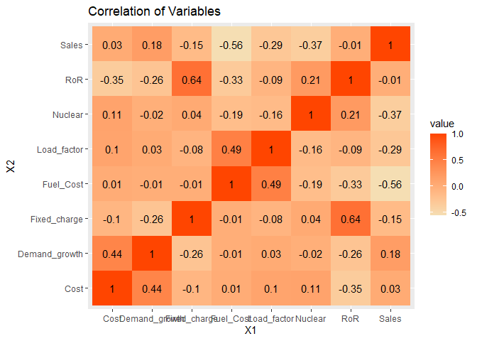
###There is positive relationship between (demand_growth and
cost),(load factor and fuel cost).There is strong positive relationship
between ROR and fixed charge.There is strong negative relationship
between Sales and Fuel Cost.Inverse relationship btw demand growth and
fixed charge shows as more people use utility ,the fixed cost goes
down.Positive relationship btw fuel cost and load factor shows that for
better utility efficiency, the cost of fuel will be higher. ###PCA
Utilities.df <- setDF(Utilities_dt)
pcs8 <- prcomp(na.omit(Utilities.df[,-c(1)]))
summary(pcs8)
## Importance of components:
## PC1 PC2 PC3 PC4 PC5 PC6 PC7
## Standard deviation 3549.9901 41.26913 15.49215 4.001 2.783 1.977 0.3501
## Proportion of Variance 0.9998 0.00014 0.00002 0.000 0.000 0.000 0.0000
## Cumulative Proportion 0.9998 0.99998 1.00000 1.000 1.000 1.000 1.0000
## PC8
## Standard deviation 0.1224
## Proportion of Variance 0.0000
## Cumulative Proportion 1.0000
pcs8$rot## PC1 PC2 PC3 PC4
## Fixed_charge 7.883140e-06 -0.0004460932 0.0001146357 -0.0057978329
## RoR 6.081397e-06 -0.0186257078 0.0412535878 0.0292444838
## Cost -3.247724e-04 0.9974928360 -0.0566502956 -0.0179103135
## Load_factor 3.618357e-04 0.0111104272 -0.0964680806 0.9930009368
## Demand_growth -1.549616e-04 0.0326730808 -0.0038575008 0.0544730799
## Sales -9.999983e-01 -0.0002209801 0.0017377455 0.0005270008
## Nuclear 1.767632e-03 0.0589056695 0.9927317841 0.0949073699
## Fuel_Cost 8.780470e-05 0.0001659524 -0.0157634569 0.0276496391
## PC5 PC6 PC7 PC8
## Fixed_charge 0.0198566131 -0.0583722527 -1.002990e-01 9.930280e-01
## RoR 0.2028309717 -0.9735822744 -5.984233e-02 -6.717166e-02
## Cost 0.0355836487 -0.0144563569 -9.986723e-04 -1.312104e-03
## Load_factor 0.0495177973 0.0333700701 2.930752e-02 9.745357e-03
## Demand_growth -0.9768581322 -0.2038187556 8.898790e-03 8.784363e-03
## Sales 0.0001471164 0.0001237088 -9.721241e-05 5.226863e-06
## Nuclear -0.0057261758 0.0430954352 -1.043775e-02 2.059461e-03
## Fuel_Cost -0.0215054038 0.0633116915 -9.926283e-01 -9.594372e-02
###From standard PCAs analysis,we get to know that PC1 and PC2 can give us the values required for correct analysis of the data. So,We can drop rest of the variables as we have already reached 99% of the cumulative proportion.We are just considering one variable for dimension reduction analysis
####Normalised PCAs
pcs.cor <- prcomp(na.omit(Utilities.df[,-c(1)]), scale. = T)
summary(pcs.cor)
## Importance of components:
## PC1 PC2 PC3 PC4 PC5 PC6 PC7
## Standard deviation 1.4741 1.3785 1.1504 0.9984 0.80562 0.75608 0.46530
## Proportion of Variance 0.2716 0.2375 0.1654 0.1246 0.08113 0.07146 0.02706
## Cumulative Proportion 0.2716 0.5091 0.6746 0.7992 0.88031 0.95176 0.97883
## PC8
## Standard deviation 0.41157
## Proportion of Variance 0.02117
## Cumulative Proportion 1.00000
pcs.cor$rot## PC1 PC2 PC3 PC4 PC5
## Fixed_charge 0.44554526 -0.23217669 0.06712849 -0.55549758 0.4008403
## RoR 0.57119021 -0.10053490 0.07123367 -0.33209594 -0.3359424
## Cost -0.34869054 0.16130192 0.46733094 -0.40908380 0.2685680
## Load_factor -0.28890116 -0.40918419 -0.14259793 -0.33373941 -0.6800711
## Demand_growth -0.35536100 0.28293270 0.28146360 -0.39139699 -0.1626375
## Sales 0.05383343 0.60309487 -0.33199086 -0.19086550 -0.1319721
## Nuclear 0.16797023 -0.08536118 0.73768406 0.33348714 -0.2496462
## Fuel_Cost -0.33584032 -0.53988503 -0.13442354 -0.03960132 0.2926660
## PC6 PC7 PC8
## Fixed_charge -0.00654016 0.20578234 -0.48107955
## RoR -0.13326000 -0.15026737 0.62855128
## Cost 0.53750238 -0.11762875 0.30294347
## Load_factor 0.29890373 0.06429342 -0.24781930
## Demand_growth -0.71916993 -0.05155339 -0.12223012
## Sales 0.14953365 0.66050223 0.10339649
## Nuclear 0.02644086 0.48879175 -0.08466572
## Fuel_Cost -0.25235278 0.48914707 0.43300956
###From Normalised PCAs,since all variables are considered for the dimension reduction analysis so the changes in cumultive proprtion is gradually increasing.In this we need to consider PC1 to PC7 for better results.
