PSITIP

Python Symbolic Information Theoretic Inequality Prover

Click one of the following to run PSITIP on the browser:

>> Learn Information Theory with PSITIP (Jupyter Binder) <<

>> Learn Information Theory with PSITIP (Google Colab) <<

Click here for the Installation Guide for local installation

PSITIP is a computer algebra system for information theory written in Python. Random variables, expressions and regions are objects in Python that can be manipulated easily. Moreover, it implements a versatile deduction system for automated theorem proving. PSITIP supports features such as:

Proving linear information inequalities via the linear programming method by Yeung and Zhang (see References). The linear programming method was first implemented in the ITIP software developed by Yeung and Yan ( http://user-www.ie.cuhk.edu.hk/~ITIP/ ).
Automated inner and outer bounds for multiuser settings in network information theory. PSITIP is capable of proving 57.1% (32 out of 56) of the theorems in Chapters 1-14 of Network Information Theory by El Gamal and Kim. (See the Jupyter Notebook examples ).
Proving and discovering entropy inequalities in additive combinatorics, e.g. the entropy forms of Ruzsa triangle inequality and sum-difference inequality [Ruzsa 1996], [Tao 2010]. (See the Jupyter Notebook examples ).
Proving first-order logic statements on random variables (involving arbitrary combinations of information inequalities, existence, for all, and, or, not, implication, etc).
Numerical optimization over distributions, and evaluation of rate regions involving auxiliary random variables (e.g. Example 1: Degraded broadcast channel).
Interactive mode and Parsing LaTeX code.
Finding examples of distributions where a set of constraints is satisfied.
Fourier-Motzkin elimination.
Discover inequalities via the convex hull method for polyhedron projection [Lassez-Lassez 1991].
Non-Shannon-type inequalities.
Integration with Jupyter Notebook and LaTeX output.
Generation of Human-readable Proof.
Drawing Information diagrams.
User-defined information quantities (see Real-valued information quantities, e.g. information bottleneck, and Wyner's CI and Gács-Körner CI in the example below).
Bayesian network optimization. PSITIP is optimized for random variables following a Bayesian network structure, which can greatly improve performance.
(Experimental) Quantum information theory and von Neumann entropy.

Examples with Jupyter Notebook (ipynb file) :

%matplotlib inline
from psitip import *
PsiOpts.setting(
    solver = "ortools.GLOP",    # Set linear programming solver
    str_style = "std",          # Conventional notations in output
    proof_note_color = "blue",  # Reasons in proofs are blue
    solve_display_reg = True,   # Display claims in solve commands
    random_seed = 4321          # Random seed for example searching
)

X, Y, Z, W, U, V, M, S = rv("X, Y, Z, W, U, V, M, S") # Declare random variables

H(X+Y) - H(X) - H(Y)  # Simplify H(X,Y) - H(X) - H(Y)

bool(H(X) + I(Y & Z | X) >= I(Y & Z))  # Check H(X) + I(Y;Z|X) >= I(Y;Z)

True

# Prove an implication
(markov(X+W, Y, Z) >> (I(X & W | Y) / 2 <= H(X | Z))).solve(full=True)

# Information diagram that shows the above implication
(markov(X+W, Y, Z) >> (I(X & W | Y) / 2 <= H(X | Z))).venn()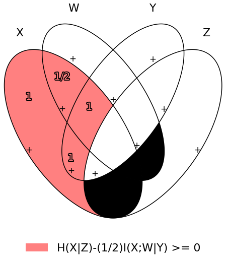

# Disprove an implication by a counterexample
(markov(X+W, Y, Z) >> (I(X & W | Y) * 3 / 2 <= H(X | Z))).solve(full=True)

# The condition "there exists Y independent of X such that 
# X-Y-Z forms a Markov chain" can be simplified to "X,Z independent"
(markov(X, Y, Z) & indep(X, Y)).exists(Y).simplified()

Additive combinatorics

A, B, C = rv("A, B, C", alg="abelian")  # Abelian-group-valued RVs

# Entropy of sum (or product) is submodular [Madiman 2008]
(indep(A, B, C) >> (H(A*B*C) + H(B) <= H(A*B) + H(B*C))).solve(full=True)

# Entropy form of Ruzsa triangle inequality [Ruzsa 1996], [Tao 2010]
(indep(A, B, C) >> (H(A/C) <= H(A/B) + H(B/C) - H(B))).solve(full=True)

User-defined information quantities

# Define Gács-Körner common information [Gács-Körner 1973]
gkci = ((H(V|X) == 0) & (H(V|Y) == 0)).maximum(H(V), V)

# Define Wyner's common information [Wyner 1975]
wci = markov(X, U, Y).minimum(I(U & X+Y), U)

# Define common entropy [Kumar-Li-El Gamal 2014]
eci = markov(X, U, Y).minimum(H(U), U)

(gkci <= I(X & Y)).solve()        # Gács-Körner <= I(X;Y)

(I(X & Y) <= wci).solve()         # I(X;Y) <= Wyner

(wci <= emin(H(X), H(Y))).solve() # Wyner <= min(H(X),H(Y))

(gkci <= wci).solve(full=True) # Output proof of Gács-Körner <= Wyner

# Automatically discover inequalities among quantities
universe().discover([X, Y, gkci, wci, eci])

Automatic inner/outer bound for degraded broadcast channel

X, Y, Z = rv("X, Y, Z")
M1, M2 = rv_array("M", 1, 3)
R1, R2 = real_array("R", 1, 3)

model = CodingModel()
model.add_node(M1+M2, X, label="Enc")  # Encoder maps M1,M2 to X
model.add_edge(X, Y)                   # Channel X -> Y -> Z
model.add_edge(Y, Z)
model.add_node(Y, M1, label="Dec 1")   # Decoder1 maps Y to M1
model.add_node(Z, M2, label="Dec 2")   # Decoder2 maps Z to M2
model.set_rate(M1, R1)                 # Rate of M1 is R1
model.set_rate(M2, R2)                 # Rate of M2 is R2

model.graph()             # Draw diagram

# Inner bound via [Lee-Chung 2015], give superposition region [Bergmans 1973], [Gallager 1974]
r = model.get_inner(is_proof=True)  # Display codebook, encoding and decoding info
r.display(note=True)

# Automatic outer bound with 1 auxiliary, gives superposition region
model.get_outer(1)

# Converse proof, print auxiliary random variables
(model.get_outer() >> r).solve(display_reg=False)

# Output the converse proof
(model.get_outer(is_proof = True) >> r).proof()

r.maximum(R1 + R2, [R1, R2])          # Max sum rate

r.maximum(emin(R1, R2), [R1, R2])     # Max symmetric rate

r.exists(R1)   # Eliminate R1, same as r.projected(R2)

# Eliminate Z, i.e., taking union of the region over all choices of Z
# The program correctly deduces that it suffices to consider Z = Y
r.exists(Z).simplified()

Non-Shannon-type Inequalities

# Zhang-Yeung inequality [Zhang-Yeung 1998] cannot be proved by Shannon-type inequalities
(2*I(Z&W) <= I(X&Y) + I(X & Z+W) + 3*I(Z&W | X) + I(Z&W | Y)).solve()

# Using copy lemma [Zhang-Yeung 1998], [Dougherty-Freiling-Zeger 2011]
# You may use the built-in "with copylem().assumed():" instead of the below
with eqdist([X, Y, U], [X, Y, Z]).exists(U).forall(X+Y+Z).assumed():

    # Prove Zhang-Yeung inequality, and print how the copy lemma is used
    display((2*I(Z&W) <= I(X&Y) + I(X & Z+W) + 3*I(Z&W | X) + I(Z&W | Y)).solve())

# State the copy lemma
r = eqdist([X, Y, U], [X, Y, Z]).exists(U)

# Automatically discover non-Shannon-type inequalities using copy lemma
r.discover([X, Y, Z, W]).simplified()

|

>>>> Click here for more examples (Jupyter Binder) (Google Colab) <<<<

|

About

Author: Cheuk Ting Li ( https://www.ie.cuhk.edu.hk/people/ctli.shtml ). The source code of PSITIP is released under the GNU General Public License v3.0 ( https://www.gnu.org/licenses/gpl-3.0.html ). The author would like to thank Raymond W. Yeung and Chandra Nair for their invaluable comments.

The working principle of PSITIP (existential information inequalities) is described in the following article:

C. T. Li, "An Automated Theorem Proving Framework for Information-Theoretic Results," in IEEE Transactions on Information Theory, vol. 69, no. 11, pp. 6857-6877, Nov. 2023, doi: 10.1109/TIT.2023.3296597. (Paper) (Preprint)

If you find PSITIP useful in your research, please consider citing the above article.

|

WARNING

This program comes with ABSOLUTELY NO WARRANTY. This program is a work in progress, and bugs are likely to exist. The deduction system is incomplete, meaning that it may fail to prove true statements (as expected in most automated deduction programs). On the other hand, declaring false statements to be true should be less common. If you encounter a false accept in PSITIP, please let the author know.

|

Installation Guide

To install PSITIP with its dependencies, use one of the following three options:

A. Default installation

Run (you might need to use python -m pip or py -m pip instead of pip):

pip install psitip

If you encounter an error when building pycddlib on Linux, refer to https://pycddlib.readthedocs.io/en/latest/quickstart.html#installation .

This will install PSITIP with default dependencies. The default solver is ortools.GLOP. If you want to choose which dependencies to install, or if you encounter an error, use one of the following two options instead.

B. Installation with conda (recommended)

Install Python via Anaconda (https://www.anaconda.com/).

Open Anaconda prompt and run:

conda install -c conda-forge glpk
conda install -c conda-forge pulp
conda install -c conda-forge pyomo
conda install -c conda-forge lark-parser
pip install ortools
pip install pycddlib
pip install --no-deps psitip

If you encounter an error when building pycddlib on Linux, refer to https://pycddlib.readthedocs.io/en/latest/quickstart.html#installation .
(Optional) Graphviz (https://graphviz.org/) is required for drawing Bayesian networks and communication network model. It can be installed via conda install -c conda-forge python-graphviz
(Optional) If numerical optimization is needed, also install PyTorch (https://pytorch.org/).

C. Installation with pip

Install Python (https://www.python.org/downloads/).

Run (you might need to use python -m pip or py -m pip instead of pip):

pip install numpy
pip install scipy
pip install matplotlib
pip install ortools
pip install pulp
pip install pyomo
pip install lark-parser
pip install pycddlib
pip install --no-deps psitip

If you encounter an error when building pycddlib on Linux, refer to https://pycddlib.readthedocs.io/en/latest/quickstart.html#installation .
(Optional) The GLPK LP solver can be installed on https://www.gnu.org/software/glpk/ or via conda.
(Optional) Graphviz (https://graphviz.org/) is required for drawing Bayesian networks and communication network model. A Python binding can be installed via pip install graphviz
(Optional) If numerical optimization is needed, also install PyTorch (https://pytorch.org/).

|

Basics

The following classes and functions are in the psitip module. Use from psitip import * to avoid having to type psitip.something every time you use one of these functions.

Random variables are declared as X = rv("X"). The name "X" passed to "rv" must be unique. Variables with the same name are treated as being the same. The return value is a Comp object (compound random variable).

As a shorthand, you may declare multiple random variables in the same line as X, Y = rv("X, Y"). Variable names are separated by ", ".

The joint random variable (X,Y) is expressed as X + Y (a Comp object).
Entropy H(X) is expressed as H(X). Conditional entropy H(XZ) is expressed as I(X & Y | Z). The return values are Expr objects (expressions).

Joint entropy can be expressed as H(X+Y) (preferred) or H(X, Y). One may also write expressions like I(X+Y & Z+W | U+V) (preferred) or I(X,Y & Z,W | U,V).

Real variables are declared as a = real("a"). The return value is an Expr object (expression).
Expressions can be added and subtracted with each other, and multiplied and divided by scalars, e.g. I(X + Y & Z) * 3 - a * 4.

While PSITIP can handle affine expressions like H(X) + 1 (i.e., adding or subtracting a constant), affine expressions are unrecommended as they are prone to numerical error in the solver.

While expressions can be multiplied and divided by each other (e.g. H(X) * H(Y)), most symbolic capabilities are limited to linear and affine expressions. Numerical only: non-affine expressions can be used in concrete models, and support automated gradient for numerical optimization tasks, but do not support most symbolic capabilities for automated deduction.

We can take power (e.g. H(X) ** H(Y)) and logarithm (using the elog function, e.g. elog(H(X) + H(Y))) of expressions. Numerical only: non-affine expressions can be used in concrete models, and support automated gradient for numerical optimization tasks, but do not support most symbolic capabilities for automated deduction.

When two expressions are compared (using <=, >= or ==), the return value is a Region object (not a bool). The Region object represents the set of distributions where the condition is satisfied. E.g. I(X & Y) == 0, H(X | Y) <= H(Z) + a.

~a is a shorthand for a == 0 (where a is an Expr). The reason for this shorthand is that not a is the same as a == 0 for a being int/float in Python. For example, the region where Y is a function of X (both Comp) can be expressed as ~H(Y|X).

While PSITIP can handle general affine and half-space constraints like H(X) <= 1 (i.e., comparing an expression with a nonzero constant, or comparing affine expressions), they are unrecommended as they are prone to numerical error in the solver.

While PSITIP can handle strict inequalities like H(X) > H(Y), strict inequalities are unrecommended as they are prone to numerical error in the solver.

The intersection of two regions (i.e., the region where the conditions in both regions are satisfied) can be obtained using the "&" operator. E.g. (I(X & Y) == 0) & (H(X | Y) <= H(Z) + a).

To build complicated regions, it is often convenient to declare r = universe() (universe() is the region without constraints), and add constraints to r by, e.g., r &= I(X & Y) == 0.

The union of two regions can be obtained using the "|" operator. E.g. (I(X & Y) == 0) | (H(X | Y) <= H(Z) + a). (Note that the return value is a RegionOp object, a subclass of Region.)
The complement of a region can be obtained using the "~" operator. E.g. ~(H(X | Y) <= H(Z) + a). (Note that the return value is a RegionOp object, a subclass of Region.)
The Minkowski sum of two regions (with respect to their real variables) can be obtained using the "+" operator.
A region object can be converted to bool, returning whether the conditions in the region can be proved to be true (using Shannon-type inequalities). E.g. bool(H(X) >= I(X & Y)).
The constraint that X, Y, Z are mutually independent is expressed as indep(X, Y, Z) (a Region object). The function indep can take any number of arguments.

The constraint that X, Y, Z are mutually conditionally independent given W is expressed as indep(X, Y, Z).conditioned(W).

The constraint that X, Y, Z forms a Markov chain is expressed as markov(X, Y, Z) (a Region object). The function markov can take any number of arguments.
The constraint that X, Y, Z are informationally equivalent (i.e., contain the same information) is expressed as equiv(X, Y, Z) (a Region object). The function equiv can take any number of arguments. Note that equiv(X, Y) is the same as (H(X|Y) == 0) & (H(Y|X) == 0).
The rv_seq method constructs a sequence of random variables. For example, X = rv_seq("X", 10) gives a Comp object consisting of X0, X1, ..., X9.

A sequence can be used by itself to represent the joint random variable of the variables in the sequence. For example, H(X) gives H(X0,...,X9).

A sequence can be indexed using X[i] (returns a Comp object). The slice notation in Python also works, e.g., X[5:-1] gives X5,X6,X7,X8 (a Comp object).

The region where the random variables in the sequence are mutually independent can be given by indep(*X). The region where the random variables form a Markov chain can be given by markov(*X).

Simplification Expr and Region objects have a simplify() method, which simplifies the expression/region in place. The simplified() method returns the simplified expression/region without modifying the object. For example, (H(X+Y) - H(X) - H(Y)).simplified() gives -I(Y & X).

Note that calling Region.simplify() can take some time for the detection of redundant constraints. Use Region.simplify_quick() instead to skip this step.

Use r.simplify(level = ???) to specify the simplification level (integer in 0,...,10). A higher level takes more time. The context manager PsiOpts.setting(simplify_level = ???): has the same effect.

The simplify method always tries to convert the region to an equivalent form which is weaker a priori (e.g. removing redundant constraints and converting equality constraints to inequalities if possible). If a stronger form is desired, use r.simplify(strengthen = True).

Logical implication. To test whether the conditions in region r1 imply the conditions in region r2 (i.e., whether r1 is a subset of r2), use r1.implies(r2) (which returns bool). E.g. (I(X & Y) == 0).implies(H(X + Y) == H(X) + H(Y)).

Use r1.implies(r2, aux_hull = True) to allow rate splitting for auxiliary random variables, which may help proving the implication. This takes considerable computation time.

Use r1.implies(r2, level = ???) to specify the simplification level (integer in 0,...,10), which may help proving the implication. A higher level takes more time.

Logical equivalence. To test whether the region r1 is equivalent to the region r2, use r1.equiv(r2) (which returns bool). This uses implies internally, and the same options can be used.
Use str(x) to convert x (a Comp, Expr or Region object) to string. The tostring method of Comp, Expr and Region provides more options. For example, r.tostring(tosort = True, lhsvar = R) converts the region r to string, sorting all terms and constraints, and putting the real variable R to the left hand side of all expressions (and the rest to the right).
(Warning: experimental) Quantum information theory. To use von Neumann entropy instead of Shannon entropy, add the line PsiOpts.setting(quantum = True) to the beginning. Only supports limited functionalities (e.g. verifying inequalities and implications). Uses the basic inequalities in [Pippenger 2003].

|

Advanced

Group-valued random variables are declared as X = rv("X", alg="group"). Choices of the parameter alg are "semigroup", "group", "abelian" (abelian group), "torsionfree" (torsion-free abelian group), "vector" (vector space over reals), and "real".

Multiplication is denoted as X * Y. Power is denoted as X**3. Inverse is denoted as 1 / X.

Group operation is denoted by multiplication, even for (the additive group of) vectors and real numbers. E.g. for vectors X, Y, denote X + 2Y by X * Y**2. For real numbers, X * Y means X + Y, and actual multiplication between real numbers is not supported.

Existential quantification is represented by the exists method of Region (which returns a Region). For example, the condition "there exists auxiliary random variable U such that R <= I(U;Y) - I(U;S) and U-(X,S)-Y forms a Markov chain" (as in Gelfand-Pinsker theorem) is represented by:
```
((R <= I(U & Y) - I(U & S)) & markov(U, X+S, Y)).exists(U) 
```

Calling exists on real variables will cause the variable to be eliminated by Fourier-Motzkin elimination. Currently, calling exists on real variables for a region obtained from material implication is not supported.

Calling exists on random variables will cause the variable to be marked as auxiliary (dummy).

Calling exists on random variables with the option method = "real" will cause all information quantities about the random variables to be treated as real variables, and eliminated using Fourier-Motzkin elimination. Those random variables will be absent in the resultant region (not even as auxiliary random variables). E.g.:
(indep(X+Z, Y) & markov(X, Y, Z)).exists(Y, method = "real")
gives { I(Z;X) == 0 }. Note that using method = "real" can be extremely slow if the number of random variables is more than 5, and may enlarge the region since only Shannon-type inequalities are enforced.
Calling exists on random variables with the option method = "ci" will apply semi-graphoid axioms for conditional independence implication [Pearl-Paz 1987], and remove all inequalities about the random variables which are not conditional independence constraints. Those random variables will be absent in the resultant region (not even as auxiliary random variables). This may enlarge the region.

Material implication between Region is denoted by the operator >>, which returns a Region object. The region r1 >> r2 represents the condition that r2 is true whenever r1 is true. Note that r1 >> r2 is equivalent to ~r1 | r2, and r1.implies(r2) is equivalent to bool(r1 >> r2).

Material equivalence is denoted by the operator ==, which returns a Region object. The region r1 == r2 represents the condition that r2 is true if and only if r1 is true.

Universal quantification is represented by the forall method of Region (which returns a Region). This is usually called after the implication operator >>. For example, the condition "for all U such that U-X-(Y1,Y2) forms a Markov chain, we have I(U;Y1) >= I(U;Y2)" (less noisy broadcast channel [Körner-Marton 1975]) is represented by:
```
(markov(U,X,Y1+Y2) >> (I(U & Y1) >= I(U & Y2))).forall(U)
```

Calling forall on real variables is supported, e.g. (((R == H(X)) | (R == H(Y))) >> (R == H(Z))).forall(R) gives (H(X) == H(Z)) & (H(Y) == H(Z)).

Ordering of forall and exists among random variables are respected, i.e., r.exists(X1).forall(X2) is different from r.forall(X2).exists(X1). Ordering of forall and exists among real variables are also respected. Nevertheless, ordering between random variables and real variables are not respected, and real variables are always processed first (e.g., it is impossible to have (H(X) - H(Y) == R).exists(X+Y).forall(R), since it will be interpreted as (H(X) - H(Y) == R).forall(R).exists(X+Y)).

Uniqueness is represented by the unique method of Region (which returns a Region). For example, to check that if X, Y are perfectly resolvable [Prabhakaran-Prabhakaran 2014], then their common part is unique:
```
print(bool(((H(U | X)==0) & (H(U | Y)==0) & markov(X, U, Y)).unique(U)))
```

Uniqueness does not imply existence. For both existence and uniqueness, use Region.exists_unique.

To check whether a variable / expression / constraint x (Comp, Expr or Region object) appears in y (Comp, Expr or Region object), use x in y.
To obtain all random variables (excluding auxiliaries) in x (Expr or Region object), use x.rvs. To obtain all real variables in x (Expr or Region object), use x.reals. To obtain all existentially-quantified (resp. universally-quantified) auxiliary random variables in x (Region object), use x.aux (resp. x.auxi).
Substitution. The function call r.subs(x, y) (where r is an Expr or Region, and x, y are either both Comp or both Expr) returns an expression/region where all appearances of x in r are replaced by y. To replace x1 by y1, and x2 by y2, use r.subs({x1: y1, x2: y2}) or r.subs(x1 = y1, x2 = y2) (the latter only works if x1 has name "x1").

Call subs_aux instead of subs to stop treating x as an auxiliary in the region r (useful in substituting a known value of an auxiliary).

Minimization / maximization over an expression expr over variables v (Comp, Expr, or list of Comp and/or Expr) subject to the constraints in region r is represented by the r.minimum(expr, v) / r.maximum(expr, v) respectively (which returns an Expr object). For example, Wyner's common information [Wyner 1975] is represented by:
```
markov(X, U, Y).minimum(I(U & X+Y), U)
```

It is simple to define new information quantities. For example, to define the information bottleneck [Tishby-Pereira-Bialek 1999]:

def info_bot(X, Y, t):
    U = rv("U")
    return (markov(U, X, Y) & (I(X & U) <= t)).maximum(I(Y & U), U)

X, Y = rv("X, Y")
t1, t2 = real("t1, t2")

# Check that info bottleneck is non-decreasing
print(bool((t1 <= t2) >> (info_bot(X, Y, t1) <= info_bot(X, Y, t2)))) # True

# Check that info bottleneck is a concave function of t
print(info_bot(X, Y, t1).isconcave()) # True

# It is not convex in t
print(info_bot(X, Y, t1).isconvex()) # False

The minimum / maximum of two (or more) Expr objects is represented by the emin / emax function respectively. For example, bool(emin(H(X), H(Y)) >= I(X & Y)) returns True.
The absolute value of an Expr object is represented by the abs function. For example, bool(abs(H(X) - H(Y)) <= H(X) + H(Y)) returns True.
The projection of a Region r onto the real variable a is given by r.projected(a). All real variables in r other than a will be eliminated. For projection along the diagonal a + b, use r.projected(c == a + b) (where a, b, c are all real variables, and c is a new real variable not in r). To project onto multiple coordinates, use r.projected([a, b]) (where a, b are Expr objects for real variables, or Region objects for linear combinations of real variables). For example:
```
# Multiple access channel capacity region without time sharing [Ahlswede 1971]
r = indep(X, Y) & (R1 <= I(X & Z | Y)) & (R2 <= I(Y & Z | X)) & (R1 + R2 <= I(X+Y & Z))

print(r.projected(R1))
# Gives ( ( R1 <= I(X&Z+Y) ) & ( I(X&Y) == 0 ) )

print(r.projected(R == R1 + R2)) # Project onto diagonal to get sum rate
# Gives ( ( R <= I(X+Y&Z) ) & ( I(X&Y) == 0 ) )
```
See Fourier-Motzkin elimination for another example. For a projection operation that also eliminates random variables, see Discover inequalities.
While one can check the conditions in r (a Region object) by calling bool(r), to also obtain the auxiliary random variables, instead call r.solve(), which returns a list of pairs of Comp objects that gives the auxiliary random variable assignments (returns None if bool(r) is False). For example:
```
res = (markov(X, U, Y).minimum(I(U & X+Y), U) <= H(X)).solve()
```
returns U := X. Note that res is a CompArray object, and its content can be accessed via res[U] (which gives X) or (res[0,0],res[0,1]) (which gives (U,X)).

If branching is required (e.g. for union of regions), solve may give a list of lists of pairs, where each list represents a branch. For example:
(markov(X, U, Y).minimum(I(U & X+Y), U) <= emin(H(X),H(Y))).solve()
returns [[(U, X)], [(U, Y)]].

Proving / disproving a region. To automatically prove r (a Region object) or disprove it using a counterexample, use r.solve(full = True). Loosely speaking, it will call r.solve(), (~r).example(), (~r).solve() and r.example() in this sequence to try to prove / find counterexample / disprove / find example respectively. This is extremely slow, and should be used only for simple statements.

To perform only one of the aforementioned four operations, use r.solve(method = "c") / r.solve(method = "-e") / r.solve(method = "-c") / r.solve(method = "e") respectively.

To draw the Bayesian network of a region r, use r.graph() (which gives a Graphviz digraph). To draw the Bayesian network only on the random variables in a (Comp object), use r.graph(a).
The meet or Gács-Körner common part [Gács-Körner 1973] between X and Y is denoted as meet(X, Y) (a Comp object).
The minimal sufficient statistic of X about Y is denoted as mss(X, Y) (a Comp object).
The random variable given by the strong functional representation lemma [Li-El Gamal 2018] applied on X, Y (Comp objects) with a gap term logg (Expr object) is denoted as sfrl_rv(X, Y, logg) (a Comp object). If the gap term is omitted, this will be the ordinary functional representation lemma [El Gamal-Kim 2011].
To set a time limit to a block of code, start the block with with PsiOpts(timelimit = "1h30m10s100ms"): (e.g. for a time limit of 1 hour 30 minutes 10 seconds 100 milliseconds). This is useful for time-consuming tasks, e.g. simplification and optimization.
Stopping signal file. To stop the execution of a block of code upon the creation of a file named "stop_file.txt", start the block with with PsiOpts(stop_file = "stop_file.txt"):. This is useful for functions with long and unpredictable running time (creating the file would stop the function and output the results computed so far).

|

References

The general method of using linear programming for solving information theoretic inequality is based on the following work:

R. W. Yeung, "A new outlook on Shannon's information measures," IEEE Trans. Inform. Theory, vol. 37, pp. 466-474, May 1991.
R. W. Yeung, "A framework for linear information inequalities," IEEE Trans. Inform. Theory, vol. 43, pp. 1924-1934, Nov 1997.
Z. Zhang and R. W. Yeung, "On characterization of entropy function via information inequalities," IEEE Trans. Inform. Theory, vol. 44, pp. 1440-1452, Jul 1998.
S. W. Ho, L. Ling, C. W. Tan, and R. W. Yeung, "Proving and disproving information inequalities: Theory and scalable algorithms," IEEE Transactions on Information Theory, vol. 66, no. 9, pp. 5522–5536, 2020.

There are several other pieces of software based on the linear programming approach in ITIP, for example, Xitip, FME-IT, Minitip, Citip, AITIP, CAI, and ITTP (which uses an axiomatic approach instead).

We remark that there is a Python package for discrete information theory called dit ( https://github.com/dit/dit ), which contains a collection of numerical optimization algorithms for information theory. Though it is not for proving information theoretic results.

Convex hull method for polyhedron projection:

C. Lassez and J.-L. Lassez, Quantifier elimination for conjunctions of linear constraints via a convex hull algorithm, IBM Research Report, T.J. Watson Research Center, RC 16779 (1991)

General coding theorem for network information theory:

Si-Hyeon Lee and Sae-Young Chung, "A unified approach for network information theory," 2015 IEEE International Symposium on Information Theory (ISIT), IEEE, 2015.
Si-Hyeon Lee and Sae-Young Chung, "A unified random coding bound," IEEE Transactions on Information Theory, vol. 64, no. 10, pp. 6779–6802, 2018.

Semi-graphoid axioms for conditional independence implication:

Judea Pearl and Azaria Paz, "Graphoids: a graph-based logic for reasoning about relevance relations", Advances in Artificial Intelligence (1987), pp. 357--363.

Basic inequalities of quantum information theory:

Pippenger, Nicholas. "The inequalities of quantum information theory." IEEE Transactions on Information Theory 49.4 (2003): 773-789.

Optimization algorithms:

Kraft, D. A software package for sequential quadratic programming. 1988. Tech. Rep. DFVLR-FB 88-28, DLR German Aerospace Center – Institute for Flight Mechanics, Koln, Germany.
Wales, David J.; Doye, Jonathan P. K. (1997). "Global Optimization by Basin-Hopping and the Lowest Energy Structures of Lennard-Jones Clusters Containing up to 110 Atoms". The Journal of Physical Chemistry A. 101 (28): 5111-5116.
Hestenes, M. R. (1969). "Multiplier and gradient methods". Journal of Optimization Theory and Applications. 4 (5): 303-320.
Kingma, Diederik P., and Jimmy Ba. "Adam: A method for stochastic optimization." arXiv preprint arXiv:1412.6980 (2014).

Results used as examples above:

Peter Gács and Janos Körner. Common information is far less than mutual information.Problems of Control and Information Theory, 2(2):149-162, 1973.
A. D. Wyner. The common information of two dependent random variables. IEEE Trans. Info. Theory, 21(2):163-179, 1975.
S. I. Gel'fand and M. S. Pinsker, "Coding for channel with random parameters," Probl. Contr. and Inf. Theory, vol. 9, no. 1, pp. 19-31, 1980.
Li, C. T., & El Gamal, A. (2018). Strong functional representation lemma and applications to coding theorems. IEEE Trans. Info. Theory, 64(11), 6967-6978.
K. Marton, "A coding theorem for the discrete memoryless broadcast channel," IEEE Transactions on Information Theory, vol. 25, no. 3, pp. 306-311, May 1979.
Y. Liang and G. Kramer, "Rate regions for relay broadcast channels," IEEE Transactions on Information Theory, vol. 53, no. 10, pp. 3517-3535, Oct 2007.
Bergmans, P. "Random coding theorem for broadcast channels with degraded components." IEEE Transactions on Information Theory 19.2 (1973): 197-207.
Gallager, Robert G. "Capacity and coding for degraded broadcast channels." Problemy Peredachi Informatsii 10.3 (1974): 3-14.
J. Körner and K. Marton, Comparison of two noisy channels, Topics in Inform. Theory (ed. by I. Csiszar and P. Elias), Keszthely, Hungary (August, 1975), 411-423.
El Gamal, Abbas, and Young-Han Kim. Network information theory. Cambridge University Press, 2011.
Watanabe S (1960). Information theoretical analysis of multivariate correlation, IBM Journal of Research and Development 4, 66-82.
Han T. S. (1978). Nonnegative entropy measures of multivariate symmetric correlations, Information and Control 36, 133-156.
McGill, W. (1954). "Multivariate information transmission". Psychometrika. 19 (1): 97-116.
Csiszar, Imre, and Prakash Narayan. "Secrecy capacities for multiple terminals." IEEE Transactions on Information Theory 50, no. 12 (2004): 3047-3061.
Tishby, Naftali, Pereira, Fernando C., Bialek, William (1999). The Information Bottleneck Method. The 37th annual Allerton Conference on Communication, Control, and Computing. pp. 368-377.
U. Maurer and S. Wolf. "Unconditionally secure key agreement and the intrinsic conditional information." IEEE Transactions on Information Theory 45.2 (1999): 499-514.
Wyner, Aaron, and Jacob Ziv. "The rate-distortion function for source coding with side information at the decoder." IEEE Transactions on information Theory 22.1 (1976): 1-10.
Randall Dougherty, Chris Freiling, and Kenneth Zeger. "Non-Shannon information inequalities in four random variables." arXiv preprint arXiv:1104.3602 (2011).
Imre Csiszar and Janos Körner. Information theory: coding theorems for discrete memoryless systems. Cambridge University Press, 2011.
Makarychev, K., Makarychev, Y., Romashchenko, A., & Vereshchagin, N. (2002). A new class of non-Shannon-type inequalities for entropies. Communications in Information and Systems, 2(2), 147-166.
Randall Dougherty, Christopher Freiling, and Kenneth Zeger. "Six new non-Shannon information inequalities." 2006 IEEE International Symposium on Information Theory. IEEE, 2006.
M. Vidyasagar, "A metric between probability distributions on finite sets of different cardinalities and applications to order reduction," IEEE Transactions on Automatic Control, vol. 57, no. 10, pp. 2464-2477, 2012.
A. Painsky, S. Rosset, and M. Feder, "Memoryless representation of Markov processes," in 2013 IEEE International Symposium on Information Theory. IEEE, 2013, pp. 2294-298.
M. Kovacevic, I. Stanojevic, and V. Senk, "On the entropy of couplings," Information and Computation, vol. 242, pp. 369-382, 2015.
M. Kocaoglu, A. G. Dimakis, S. Vishwanath, and B. Hassibi, "Entropic causal inference," in Thirty-First AAAI Conference on Artificial Intelligence, 2017.
F. Cicalese, L. Gargano, and U. Vaccaro, "Minimum-entropy couplings and their applications," IEEE Transactions on Information Theory, vol. 65, no. 6, pp. 3436-3451, 2019.
C. T. Li, "Efficient Approximate Minimum Entropy Coupling of Multiple Probability Distributions," arXiv preprint https://arxiv.org/abs/2006.07955 , 2020.
C. T. Li, "Infinite Divisibility of Information," arXiv preprint https://arxiv.org/abs/2008.06092 , 2020.
J. Körner and K. Marton, "Images of a set via two channels and their role in multi-user communication," IEEE Transactions on Information Theory, vol. 23, no. 6, pp. 751–761, 1977.
I. Csiszár and J. Körner, "Broadcast channels with confidential messages," IEEE transactions on information theory, vol. 24, no. 3, pp. 339–348, 1978.
Kumar and Courtade, "Which boolean functions are most informative?", ISIT 2013.
Massey, James. "Causality, feedback and directed information." Proc. Int. Symp. Inf. Theory Applic.(ISITA-90). 1990.
Renyi, Alfred (1961). "On measures of information and entropy". Proceedings of the fourth Berkeley Symposium on Mathematics, Statistics and Probability 1960. pp. 547-561.
H. O. Hirschfeld, "A connection between correlation and contingency," in Mathematical Proceedings of the Cambridge Philosophical Society, vol. 31, no. 04. Cambridge Univ Press, 1935, pp. 520-524.
H. Gebelein, "Das statistische problem der korrelation als variations-und eigenwertproblem und sein zusammenhang mit der ausgleichsrechnung," ZAMM-Journal of Applied Mathematics and Mechanics/Zeitschrift fur Angewandte Mathematik und Mechanik, vol. 21, no. 6, pp. 364-379, 1941.
A. Renyi, "On measures of dependence," Acta mathematica hungarica, vol. 10, no. 3, pp. 441-451, 1959.
Kontoyiannis, Ioannis, and Sergio Verdu. "Optimal lossless compression: Source varentropy and dispersion." 2013 IEEE International Symposium on Information Theory. IEEE, 2013.
Polyanskiy, Yury, H. Vincent Poor, and Sergio Verdu. "Channel coding rate in the finite blocklength regime." IEEE Transactions on Information Theory 56.5 (2010): 2307-2359.
Hellinger, Ernst (1909), "Neue Begründung der Theorie quadratischer Formen von unendlichvielen Veränderlichen", Journal für die reine und angewandte Mathematik, 136: 210-271.
A. El Gamal, "The capacity of a class of broadcast channels," IEEE Transactions on Information Theory, vol. 25, no. 2, pp. 166-169, 1979.
Ahlswede, Rudolf. "Multi-way communication channels." Second International Symposium on Information Theory: Tsahkadsor, Armenian SSR, Sept. 2-8, 1971.
G. R. Kumar, C. T. Li, and A. El Gamal, "Exact common information," in Proc. IEEE Symp. Info. Theory. IEEE, 2014, pp. 161-165.
V. M. Prabhakaran and M. M. Prabhakaran, "Assisted common information with an application to secure two-party sampling," IEEE Transactions on Information Theory, vol. 60, no. 6, pp. 3413-3434, 2014.
Dougherty, Randall, Chris Freiling, and Kenneth Zeger. "Non-Shannon information inequalities in four random variables." arXiv preprint arXiv:1104.3602 (2011).
F. Matus, "Infinitely many information inequalities", Proc. IEEE International Symposium on Information Theory, 2007
Dougherty, Randall, Chris Freiling, and Kenneth Zeger. "Linear rank inequalities on five or more variables." arXiv preprint arXiv:0910.0284 (2009).
A. W. Ingleton, "Representation of matroids," in Combinatorial mathematics and its applications, D. Welsh, Ed. London: Academic Press, pp. 149-167, 1971.
Madiman, Mokshay. "On the entropy of sums." 2008 IEEE Information Theory Workshop. IEEE, 2008.
Ruzsa, Imre Z. "Sums of finite sets." Number Theory: New York Seminar 1991–1995. Springer, New York, NY, 1996.
Tao, Terence. "Sumset and inverse sumset theory for Shannon entropy." Combinatorics, Probability and Computing 19.4 (2010): 603-639.

cheuktingli / psitip

PSITIP

Examples with Jupyter Notebook (ipynb file) :

Additive combinatorics

User-defined information quantities

Automatic inner/outer bound for degraded broadcast channel

Non-Shannon-type Inequalities

|

|

About

|

WARNING

|

Installation Guide

A. Default installation

B. Installation with conda (recommended)

C. Installation with pip

|

Basics

|

Advanced

|

References

About

Languages