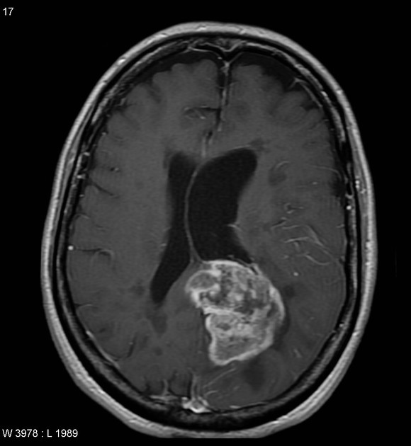
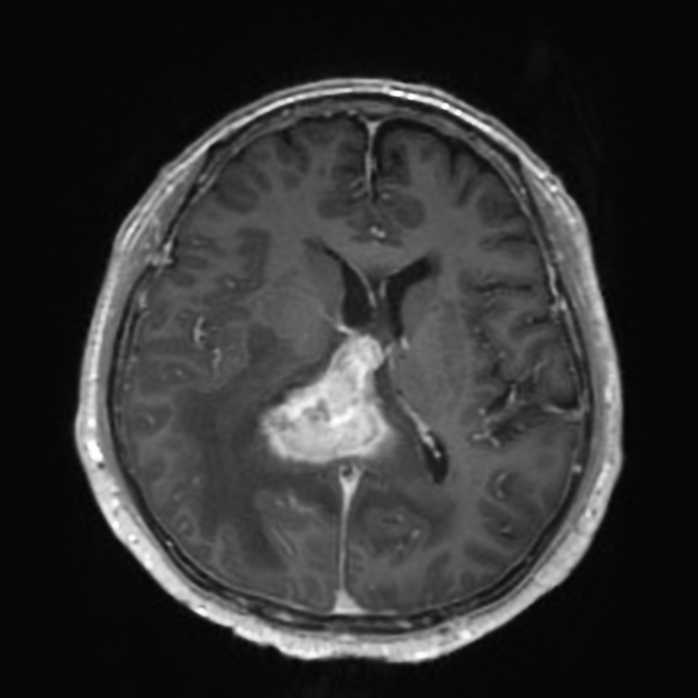
Classification of Glioblastoma versus Primary Central Nervous System Lymphoma using Convolutional Neural Networks

! CAUTION: this tool is not a medical product and is only intended for research purposes. !

Glioblastoma	Primary central nervous system lymphoma

Case courtesy of Assoc Prof Frank Gaillard, Radiopaedia.org. From the case rID: 5565.	Case courtesy of Dr Bruno Di Muzio, Radiopaedia.org. From the case rID: 64657.

Inference example

$ python step2_predict.py \
    --model-weights checkpoints/efficientnetb4_aug_none/ckpt_137_0.0000.hdf5 \
    images/sample-*.jpeg
images/sample-gbm.jpeg                   100.00 % GBM
images/sample-pcnsl.jpeg                 100.00 % PCNSL

Note: the saved models are not part of this repository. Please contact the authors for access to the models.

Steps to reproduce results

Set up Python environment. One can also use the Docker image tensorflow/tensorflow:2.5.0-gpu-jupyter. That was used to for model training. If not using a Docker image, we recommend creating a virtual environment or a conda environment for this code.
```
pip install --no-cache-dir \
    h5py \
    matplotlib \
    numpy \
    pandas \
    pillow \
    scikit-learn \
    tensorflow>=2.3.0
```
Organize data for GBM and PCNSL samples into the following directory structure. The names of the image files can be arbitrary. The most important thing is to keep GBM samples in data/gbm/ and PCNSL samples in data/pcnsl/. Note that all of these samples will be used for training and validation. A test set should be constructed with images not in this data directory.
```
data/
├── gbm
│   ├── img0.jpg
│   └── img1.jpg
└── pcnsl
    ├── img0.jpg
    └── img1.jpg
```
Convert the image data to HDF5 format. Do this with the following command:
```
python step0_convert_images_to_hdf5.py data/ data.h5
```
This will create a file data.h5 with the following datasets:
```
/gbm/380_380/features
/gbm/380_380/labels
/pcnsl/380_380/features
/pcnsl/380_380/labels
```
The 380_380 indicates that the images were resized to 380x380 pixels. The labels of GBM are 0, and the labels of PCNSL are 1.
Train models. The commands below will save checkpoints to three different directories (one for each model). The training differs by the type of augmentation applied to the training images. The the none class, no augmentation is applied. In base, images are randomly flipped, and their brightness and hue is randomly modified. In base_and_noise, images are augmented in the same way as in base but Gaussian noise is also applied to a small subset of images.
```
python step1_train_model.py \
    --augmentation none \
    --epochs 300 \
    data.h5 \
    checkpoints/augmentation-none/
```
```
python step1_train_model.py \
    --augmentation base \
    --epochs 300 \
    data.h5 \
    checkpoints/augmentation-base/
```
```
python step1_train_model.py \
    --augmentation base_and_noise \
    --epochs 300 \
    data.h5 \
    checkpoints/augmentation-baseandnoise/
```

Run inference using the trained model. Prediction is reasonably quick and does not require a GPU.

python step2_predict.py \
    --model-weights checkpoints/model.hdf5 \
    images/*

The output looks something like this:

images/sample-gbm.jpeg                   100.00 % GBM
images/sample-pcnsl.jpeg                 100.00 % PCNSL

To save the prediction results to a CSV file, use the --csv option.

python step2_predict.py \
    --csv predictions.csv \
    --model-weights checkpoints/model.hdf5 \
    images/*

The CSV file looks something like this:

path,prob_gbm,prob_pcnsl
images/sample-gbm.jpeg,0.9999999402953463,5.970465366544886e-08
images/sample-pcnsl.jpeg,4.3511390686035156e-05,0.999956488609314

Plot training metrics (loss and accuracy on training and validation sets). Use the Jupyter notebook step3_plot_training_metrics.ipynb for this.
Calculate AUROC and plot ROC curves. Use the Jupyter notebook step4_plot_roc.ipynb for this.

Plot Grad-CAM heatmaps overlaid on images.

mkdir -p gradcam-outputs
python step5_plot_grad_cam.py \
    --model-weights checkpoints/model.hdf5 \
    --output-dir gradcam-outputs \
    images/*

In Docker or Singularity

These scripts and notebooks can all be run within the official TensorFlow Docker image

tensorflow/tensorflow:2.5.0-gpu-jupyter

This Docker image can be used with Docker or Singularity.

chenxiu262 / classification-of-gbm-vs-pcnsl-using-cnns

Classification of Glioblastoma versus Primary Central Nervous System Lymphoma using Convolutional Neural Networks

Inference example

Steps to reproduce results

In Docker or Singularity

About

Languages