DynamicGrids is a generalised framework for building high-performance grid-based spatial simulations, including cellular automata, but also allowing a wider range of behaviours like random jumps and interactions between multiple grids. It is extended by Dispersal.jl for modelling organism dispersal processes.

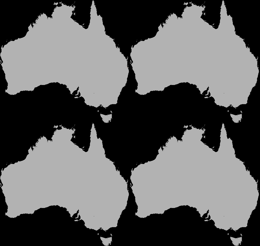
A dispersal simulation with quarantine interactions, using Dispersal.jl, custom rules and the GtkOuput from DynamicGridsGtk. Note that this is indicative of the real-time frame-rate on a laptop.

A DynamicGrids.jl simulation is run with a script like this one running the included game of life model Life():

using DynamicGrids, Crayons

init = rand(Bool, 150, 200)
output = REPLOutput(init; tspan=1:200, fps=30, color=Crayon(foreground=:red, background=:black, bold=true))
sim!(output, Life())

# Or define it from scratch (yes this is actually the whole implementation!)
const sum_states = (false, false, true, false, false, false, false, false, false), 
                   (false, false, true, true,  false, false, false, false, false)
life = Neighbors(Moore(1)) do hood, state
    sum_states[state + 1][sum(hood) + 1]
end
sim!(output, life)

A game of life simulation being displayed directly in a terminal.

Concepts

The framework is highly customisable, but there are some central ideas that define how a simulation works: grids, rules, and outputs.

Grids

Simulation grids may be any single AbstractArray or a NamedTuple of multiple AbstractArray. Usually grids contain values of Number, but other types are possible. Grids are updated by Rules that are run for every cell, at every timestep.

The init grid/s contain whatever initialisation data is required to start a simulation: the array type, size and element type, as well as providing the initial conditions:

init = rand(Float32, 100, 100)

An init grid can be attached to an Output:

output = ArrayOutput(init; tspan=1:100)

or passed in to sim!, where it will take preference over the init attached to the Output, but must be the same type and size:

sim!(output, ruleset; init=init)

For multiple grids, init is a NamedTuple of equal-sized arrays matching the names given to each Ruleset :

init = (predator=rand(100, 100), prey=(rand(100, 100))

Handling and passing of the correct grids to a Rule is automated by DynamicGrids.jl. Rules specify which grids they require in what order using the first two (R and W) type parameters, or read and write keyword arguments.

Dimensional or spatial init grids from DimensionalData.jl of GeoData.jl will propagate through the model to return output with explicit dimensions. This will plot correctly as a map using Plots.jl, to which shape files and observation points can be easily added.

Non-Number Grids

Grids containing custom and non-Number types are possible, with some caveats. They must define Base.zero for their element type, and should be a bitstype for performance. Tuple does not define zero. Array is not a bitstype, and does not define zero. SArray from StaticArrays.jl is both, and can be used as the contents of a grid. Custom structs that defne zero should also work.

However, for any multi-values grid element type, you will need to define a method of DynamicGrids.rgb that returns an ARGB32 for them to work in ImageOutputs, and isless for the REPLoutput to work.

Rules

Rules hold the parameters for running a simulation, and are applied in applyrule method that is called for each of the active cells in the grid. Rules come in a number of flavours (outlined in the docs), which allow assumptions to be made about running them that can greatly improve performance. Rules can be collected in a Ruleset, with some additional arguments to control the simulation:

ruleset = Ruleset(Life(2, 3); opt=SparseOpt())

Multiple rules can be combined in a Ruleset. Each rule will be run for the whole grid, in sequence, using appropriate optimisations depending on the parent types of each rule:

ruleset = Ruleset(rule1, rule2; timestep=Day(1), opt=SparseOpt())

For better performance (often ~2x or more), models included in a Chain object will be combined into a single model, using only one array read and write. This optimisation is limited to CellRule, or a NeighborhoodRule followed by CellRule. If the @inline compiler macro is used on all applyrule methods, all rules in a Chain will be compiled together into a single, efficient function call.

ruleset = Ruleset(rule1, Chain(rule2, rule3, rule4))

Output

Outputs are ways of storing or viewing a simulation. They can be used interchangeably depending on your needs: ArrayOutput is a simple storage structure for high performance-simulations. As with most outputs, it is initialised with the init array, but in this case it also requires the number of simulation frames to preallocate before the simulation runs.

output = ArrayOutput(init; tspan=1:10)

The REPLOutput shown above is a GraphicOutput that can be useful for checking a simulation when working in a terminal or over ssh:

output = REPLOutput(init; tspan=1:100)

ImageOutput is the most complex class of outputs, allowing full color visual simulations using ColorSchemes.jl. It can also display multiple grids using color composites or layouts, as shown above in the quarantine simulation.

DynamicGridsInteract.jl provides simulation interfaces for use in Juno, Jupyter, web pages or electron apps, with live interactive control over parameters. DynamicGridsGtk.jl is a simple graphical output for Gtk. These packages are kept separate to avoid dependencies when being used in non-graphical simulations.

Outputs are also easy to write, and high performance applications may benefit from writing a custom output to reduce memory use. Performance of DynamicGrids.jl is dominated by cache interactions, so reducing memory use has positive effects.

Example

This example implements a very simple forest fire model:

using DynamicGrids, DynamicGridsGtk, ColorSchemes, Colors

const DEAD, ALIVE, BURNING = 1, 2, 3

rule = let prob_combustion=0.0001, prob_regrowth=0.01
    Neighbors(Moore(1)) do neighborhood, cell
        if cell == ALIVE
            if BURNING in neighborhood
                BURNING
            else
                rand() <= prob_combustion ? BURNING : ALIVE
            end
        elseif cell in BURNING
            DEAD
        else
            rand() <= prob_regrowth ? ALIVE : DEAD
        end
    end
end

# Set up the init array and output (using a Gtk window)
init = fill(ALIVE, 400, 400)
processor = ColorProcessor(scheme=ColorSchemes.rainbow, zerocolor=RGB24(0.0))
output = GtkOutput(init; tspan=1:200, fps=25, minval=DEAD, maxval=BURNING, processor=processor)

# Run the simulation
sim!(output, rule)

# Save the output as a gif
savegif("forestfire.gif", output)

Timing the simulation for 200 steps, the performance is quite good:

output = ArrayOutput(init; tspan=1:200)
@time sim!(output, ruleset)
 1.384755 seconds (640 allocations: 2.569 MiB)

Alternatives

Agents.jl can also do cellular-automata style simulations. The design of Agents.jl is to iterate over a list of agents, instead of broadcasting over an array of cells. This approach is well suited to when you need to track the movement and details about individual agents throughout the simulation.

However, for simple grid models where you don't need to track individuals, like the forest fire model above, DynamicGrids.jl is two orders of magnitude faster than Agents.jl, and provides better visualisation tools. If you are doing grid-based simulation and you don't need to track individual agents, DynamicGrids.jl is probably the best tool. For other use cases, try Agents.jl.

cfoster0 / DynamicGrids.jl