pspm: Probabilistic Spatial Partition Model

Introduction

This packages contains a series of functions and classes to set up and fit a Probabilistic Spatial Partition Model and sample partitionings following the the methodology introduced by Müller-Crepon, Schvitz and Cederman (2023). In short, the model is based on a simplification of continuous geographic space as a (planar) graph. The observed partitioning is encoded on the graphs’ vertices such that each vertex is a member of one and only one partition. The graphs partitioning is modeled as the result of attractive and repulsive force active on its edges which affect the probability that the vertices they connect belong to the same or to different partitions. The model allows to estimate the effects of edge-level attributes on the repulsion/attraction between vertices, thus estimating their impact on the overall partitioning of the graph.

Please refer to the original publication for all technical details beyond the summary provided below. It can be found here and as ungated version here.

Note that our companion R-package SpatialLattice simplifies the creation and handling of spatial graphs to facilitate the analysis of spatial partitionings.

When using the pspm package, please cite:

Müller-Crepon, Carl, Guy Schvitz, Lars-Erik Cederman (2023). Shaping States into Nations: The Effects of Ethnic Geography on State Borders. American Journal of Political Science, conditionally accepted for publication.

The model

We model the distribution over all possible partitionings $P$ of lattice $G$ as a Boltzmann distribution:

$$Pr(P = p_{i}) = {e^{-\epsilon_{i}}\over\displaystyle\sum_{i = 1}^{|\mathbb{P}|}e^{-\epsilon_{i}} }$$

here, a partitioning $i$’s chance of realization decreases with its energy $\epsilon_i$. The energy of a partitioning is defined as the sum of energies on the graph’s edges that run between nodes $j$ and $k$ where $j$ and $k$ are located in the same partition ($s_{j,k} = 1$). Edges energies are not realized where $j$ and $k$ do not belong to the same partition ($s_{j,k} = 0$):

$$\epsilon_{i} = \displaystyle\sum_{j,k \in L}\, \epsilon_{j,k}\,s_{j,k}$$

Potential and realized edge-level energies are in turn affected by a constant ($\beta_0$) and a set of edge-level attributes $\textbf{x}_{j,k}$ that are weighted by a parameter vector $\beta$

$$\epsilon_{j,k} = \beta_0 + \beta\, \textbf{x}_{j,k}$$

The empirical goal of the PSPM is it to estimate parameters $\beta_0$ and $\beta$ from observed data – a positive $\beta$ indicates that an attribute exerts a repulsive force, whereas a negative one indicates an attractive force. This is due to the fact that an overal minimization of a partitings’ energy maximizes its likelihood of realization. To find the parameters that maximize this likelihood, the PSPM uses a maximum composite likelihood approach. Uncertainty estimates can be derived via a parametric bootstrap that samples partitionings with a given set of $\beta_0$ and $\beta$ parameters and then fits the model on the sampled partitionings.

Installation

You can directly download and install the pspm package from GitHub. Before doing so, please make sure that you have Python3 installed, which the package heavily relies on. For simplicity and as shown below, you can also install python and necessary modules from within R, using ’s and functions.

Upon installation and first usage, the package should automatically install all necessary python dependencies via the reticulate R-package. If this is not the case, the user may see an error and have install the following modules manually: scipy, networkx, numpy, abc, typing, collections.

# # Get python ready if not yet installed
# library(reticulate)
# reticulate::install_miniconda()
# reticulate::py_install(c("scipy","networkx"))

# Download pspm package
library(devtools)
install_github(repo = "carl-mc/pspm")

Getting started

the pspm package heavily builds on the igraph library which is used to handle the underlying network data and allows user-friendly data manipulation. Since random sampling plays an important role during sampling, it is recommended to set a random seed in R and python. pspm_set_seed() achieves just that.

# # If multiple python versions installed, point reticulate to python 3.x
# your_python_path <- '/usr/bin/python3' ## customize to your machine!
# Sys.setenv(RETICULATE_PYTHON = your_python_path)

# Packages
library(pspm)
library(igraph)

# Set seeds in R and python
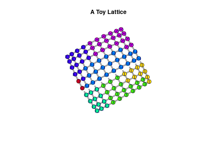
pspm_set_seed(1)

Setting up a toy lattice

To illustrate the model. we first set up a toy lattice – as a PSPM object – with 100 nodes arranges on a 10-by-10 grid. The lattice encodes two edge-level characteristics that separate one side of the lattice from the other – think of a river or mountain range. The distribution of one of these attributes is shown as dotted vs. straight edges on the graph below. Both attributes exert repulsive forces (beta = c(2,1)). Furthermore, the vertices are attracted to each other by a baseline constant of -2. We sample a partitioning of the lattice with a burn-in period of 10 rounds.

Please see the R-package SpatialLattice for code and examples on how to construct spatial graph data for observed spatial partitionings.

# Make mock PSPM Object with a sampled partitioning
sl <- generate_grid_data(N_sqrd = 10, ## 10 x 10 lattice
                        beta0 = -2, ## Negative constant = baseline attraction between nodes
                        beta = c(2,1), ## Include two repulsive edge-level predictors
                        dep_structure = "von_neumann", ## Each node connects to 4 neighbors
                        burnin = 10 ## Sample with a 10 burn-in periods
                        )

# Print class of object
print(class(sl))

## [1] "PSPM" "R6"

# Plot PSPM object
sl$plot_partitioning(edge_predictor = 1, 
                     edge.width = 5, vertex.size = 10,
                     main = "A Toy Lattice")

PSPM to igraph conversion

The PSPM object created above can be transformed into an igraph object and vice-versa using the following methods:

# Transform PSPM to igraph
graph <- PSPM2igraph(sl)

# Transfers data as edge- and vertex-attributes
edge_attr_names(graph)

## [1] "x1" "x2"

vertex_attr_names(graph)

## [1] "X1" "Y"

# Transform igraph back to PSPM
sl.from.g <- igraph2PSPM(g = graph, 
                         outcome_name = "Y",
                         edge_pred_names = c("x1", "x2"))

Fitting a PSPM Model

Finally, we can fit the PSPM to estimate the effect of the edge-level attributes on the partitioning of the lattice. The function fit_pspm_model() provides a wrapper around lower-level functions and classes, allowing the user to estimate the model directly from an igraph object with a formula where the left-handside variable Y refers to the vertex attribute that encodes vertices partition members and the right-handside variables referring to edge-level predictors. Multiple graphs can be passed to the function at the same time such that one model is fit across them. Once a model is fit, bootstrap_pspm() allows for carrying out a (parallelized) parametric bootstrap which can return the full distribution of estimates as well as (basic and percentile-based) confidence intervals.

## The easy way

### Estimate
m.simple <- fit_pspm_model(formula = Y ~ x1 + x2, 
                           g_ls = list(graph),
                           return_pspm = TRUE)

### Bootstrap CIs
bs.simple <- bootstrap_pspm(m.simple,
                            n_boot_iter = 10, ## Should be > 100
                            burnin = 10, ## Could be higher, depending on complexite of graph and model
                            cl = 10L, ## Number of CPUs for parallelization
                            return_sims = TRUE, ## Return full distribution of estimates
                            ci_level = .95)

## [1] "Load Learn Object on cluster"
## [1] "Run Bootstrap"

### Summary
summary(m.simple)

## --------------------------------------------
## Maximum Likelihood estimation
## BFGS maximization, 31 iterations
## Return code 0: successful convergence 
## Log-Likelihood: -13.44675 
## 3  free parameters
## Estimates:
##          Estimate Std. error t value  Pr(> t)    
## Constant  -2.5097     0.5919  -4.240 2.23e-05 ***
## x1         1.9450     1.8374   1.059    0.290    
## x2         0.4492     0.9306   0.483    0.629    
## ---
## Signif. codes:  0 '***' 0.001 '**' 0.01 '*' 0.05 '.' 0.1 ' ' 1
## --------------------------------------------

print(bs.simple$ci_mat)

##            Constant        x1         x2
## LB_Basic -3.3369735 1.6394587 -0.6487487
## UB_Basic -0.8817648 2.9760757  2.3140127
## LB_Perc  -4.1375785 0.9139855 -1.4156026
## UB_Perc  -1.6823697 2.2506025  1.5471588

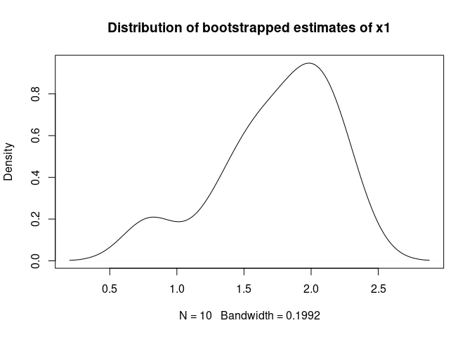
plot(density(bs.simple$beta_boot[,"x1"]),
     main = "Distribution of bootstrapped estimates of x1")

For completeness, the following code shows the same estimation process using the lower-level classes and functions in the PSPM package. We first have to transform our PSPM object into a PSPMLearn object, which include the fit_composite_log_likelihood() method. Once the PSPMLearn object is fitted, it can be directly bootstrapped using the appropriate method. Note that this method does not automatically handle missing data and other intricacies, such as keeping track of variable names.

## The complicated way (inside the wrapper)

### Initiate PSPMLearn Object
learn_obj <- PSPMLearn$new(list(sl.from.g))

### Fit
m.compl <- learn_obj$fit_composite_log_likelihood(beta_init = c(0,0,0))

### Bootstrap
bs.compl <- learn_obj$par_bootstrap_composite_log_likelihood(n_boot_iter = 10, burnin = 10,
                                                 cl = 10L, return_sims = FALSE, ci_level = .95)

## [1] "Load Learn Object on cluster"
## [1] "Run Bootstrap"

### Summary
summary(m.compl)

## --------------------------------------------
## Maximum Likelihood estimation
## BFGS maximization, 31 iterations
## Return code 0: successful convergence 
## Log-Likelihood: -13.44675 
## 3  free parameters
## Estimates:
##      Estimate Std. error t value  Pr(> t)    
## [1,]  -2.5097     0.5919  -4.240 2.23e-05 ***
## [2,]   1.9450     1.8374   1.059    0.290    
## [3,]   0.4492     0.9306   0.483    0.629    
## ---
## Signif. codes:  0 '***' 0.001 '**' 0.01 '*' 0.05 '.' 0.1 ' ' 1
## --------------------------------------------

print(bs.compl)

##            Constant        x1         x2
## LB_Basic -3.3369735 1.6394587 -0.6487487
## UB_Basic -0.8817648 2.9760757  2.3140127
## LB_Perc  -4.1375785 0.9139855 -1.4156026
## UB_Perc  -1.6823697 2.2506025  1.5471588

Producing nice tables

Finally, models fitted with fit_pspm_model() and the (maxLik)[https://cran.r-project.org/web/packages/maxLik/index.html] methods used under the hood can be printed as text, html, or latex files using a slight extension of the (texreg)[https://cran.r-project.org/web/packages/texreg/texreg.pdf] package.

# Integration with texreg
pspm2table(list(m.simple),
           bootci = list(bs.simple$ci_mat), boottype = "percentile",
           type = "text", add.stats = c("Edges" = "N_edges", "Vertices" = "N"))

## 
## ==============================
##                 Model 1       
## ------------------------------
## Constant         -2.51 *      
##                 [-4.14; -1.68]
## x1                1.95 *      
##                 [ 0.91;  2.25]
## x2                0.45        
##                 [-1.42;  1.55]
## ------------------------------
## Edges           180           
## Vertices        100           
## Log-Likelihood  -13.45        
## Num. obs.       100           
## ==============================
## * 0 outside the confidence interval.

Feedback, comments, questions

We are very grateful for any bug reports, feedback, questions, or contributions to this package. Please report any issues here or write to c.a.muller-crepon [at] lse.ac.uk .

carl-mc / pspm