callummcdougall / computational-thread-art

Code that renders an image as a series of lines connecting pins around a circular frame (for more detail, see my Medium page).

Computational Thread Art

This project contains code that renders an image as a series of lines connecting picture hooks around a circular frame. For more detail in the physical implementation of these pieces, see my article on Medium. The 4 sections in this document are:

• Algorithm description, which gives a broad picture of how the algorithm works. For more detail, see the Jupyter Notebook file (where each function is explained).
• How to run, which give instructions for generating your own output, as well as tips on what images work best.
• Algorithm Examples, where I describe how I've provided example pieces of code that you can try out.
• Final thoughts, in which I outline the future directions I might take this algorithm.

Algorithm description

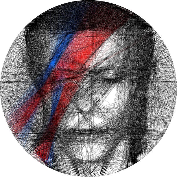
The original algorithm for rendering the actual image went as follows: first, an image is converted into a square array of greyscale pixel values from 0 to 255, where 0 represents white, and 255 black. The coordinates for the hook positions are calculated. A starting hooks is chosen, and a subset of the lines connecting that hook to other hooks are randomly chosen. Each line is tested by calculating how much it reduces the penalty (which is defined as the average of all the absolute pixel values in the image). A line will change the penalty by reducing the value of all the pixels it goes through by some fixed amount. For instance, a line through a mostly black area might change pixel values from 255 to 155 (reducing penalty a lot), whereas a line through a mostly white area - or an area which already has a lot of lines - might change pixel values from 20 to -80 (actually making the penalty worse). Once all these penalty changes have been calculated, the line which reduces the penalty the most will be chosen, the pixel values will be edited accordingly, and this process will repeat from the new hook. Once a certain number of lines have been drawn, the algorithm terminates. For the images that use colour, I usually just run the algorithm for each colour separately, using very specific images designed with photo editing software (I use GIMP). See the David Bowie lightning project for a perfect example of this.

This original algorithm has been improved significantly, primarily by making the penalty more complicated than just the absolute sum of pixel values. The actual formula for penalty is:

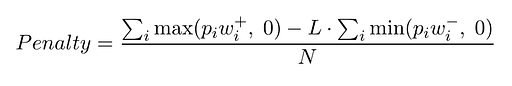
where p_i is the pixel value, w⁺ and w^- are the positive and negative importance weightings, L is the lightness penalty, N is the line norm, and the sum is taken over all pixels the line goes through.

• The lightness penalty is a value (usually between 0 and 1) which reduces the penalty for negative pixels (or to put it in terms of the actual artwork, it makes the algorithm more willing to draw too many lines than too few)
• The importance weighting is an image of the same dimensions of the original image, but when it is read by the algorithm, every pixel value is scaled to between 0 and 1, so the darker pixels indicate areas you want to give more weight to in the penalty calculation. The algorithm will prioritize accuracy in these areas at the expense of the rest of the image.
• The line norm can have 3 different values: 1 (so penalty is just total sum), number of pixels (so penalty is average per pixel), or sum of all the weightings of the pixels (so penalty is average per weighted pixel). If w⁺ and w^- are different, the latter mode defaults to using w⁺.

The second half of the code creates a Eulerian path, which is a path around the vertices that uses each edge exactly once. For this to exist, we require 2 conditions: parity (the number of lines connected to each side of the hook must be the same, since every line must enter the hook on one side and leave on the other side), and connectedness (every hook must be reachable from every other). The first thing the code does is add lines so that these 2 conditions are satistfied (these added lines go around the outside of the wheel when I make my art in real life, so they don't interfere with the image). Once this is done, then a path is iteratively built up using Hierholzer's algorithm. Essentially, this works by drawing a loop, and if there are any edges left un-drawn, it goes through the loop and finds a place where it can "stick on" another loop. If the conditions of parity and connectedness are satisfied, then we can iterate this process until all edges are connected in the same loop.

How to run

I would recommend running this algorithm in Jupyter Notebooks, or something similar (this shouldn't come as a surprise given this is how the documents are saved in this repository). Jupyter Notebooks lend themselves well to running this code; once I have selected an image I usually like to run lots of trials (tweaking the parameters, or editing the image), so the flexibility of notebooks is very useful. If you haven't downloaded Jupyter Notebooks, you can always use it in your browser (which requires a lot less effort!). To run the algorithm using your own image, you can take any of my example algorithms (see section Algorithm Examples), and replace the appropriate bits of code.

1. IMAGE PREPARATION

   1i. Have an image (either jpg or png) stored in your current working directory. It must be square in size (if it isn't, it will be squashed into shape). Here are a few tips on choosing and preparing the image:

   • The algorithm is very selective; lots of photos just aren't suitable. If you can't get a decent-looking output in the first 5 prototypes, it's probably best to try a different image.
   • Convert the image to black and white first; this helps evaluate suitability.
   • Having a high-res image isn't actually very important, usually 400px*400px will suffice.
   • If your image has a background, make sure that it is noticably different in brightness from the foreground. For instance, lots of my images have a radial gradient for the background (best example of this is the butterfly).
   • Characteristics of good images:
     • good tonal range (i.e. lots of highlights, shadows and midtones)
     • lots of long straight lines across the image (e.g. angular features if you're doing a face)
   • Characteristics of bad images:
     • low contrast
     • large white / very bright patches
     • one side of the image is in shadow (this is an especially big problem with faces) 1ii. Prepare an importance weighting (optional). This is recommended if your picture has a foreground or particular features that you want to emphasise. The importance weighting should be an edited version of the original (same size and format, no cropping). It should be greyscale, with black areas indicating the highest importance and white indicating the least importance. Here are a few tips on creating the importance weighting:
   • Beware of sharp lines in importance weightings, they can look a bit jarring. Unless your actual image has sharp lines in the same place, try to blur the edges of different sections of colour in importance weightings.
   • You can choose to have a different importance weighting for positive and negative penalties. I would recommend not using this feature unless strictly necessary, because it can lead to unforseen consequences with image quality. The only purpose I use it for is preserving small bright areas (e.g. whites of eyes), since I can make the positive weighting light on the eyes bright and the negative weighting dark (so the algorithm is fine with not drawing too few lines, but it is very reluctant to draw too many). Even in these situations, I try to keep wpos and wneg very similar.
   • Even if you care less about accuracy in the background, you should assign a small weighting too it. When I was rendering Churchill for the first time, I put 0 importance weighting on the background, and the bunching of vertical lines on either side of his face made it look like he had devil horns!

2. LINE GENERATION

   Below is an image of the Jupyter Notebook I used for my Churchill piece, showing the cells relevant for digital creation. I will go through each of the cells, and each of the parameters, in turn.

   

   • The first cell has the size parameters: the real diameter of the wheels and width of the hooks you are using (in meters), the wheel pixel size (which is the side-length of the digital image you want to create), and the number of hooks you are using. If you're just creating digital art, I would recommend leaving these settings the same as the image above (this has the added advantage that all thread vertices are evenly spaced). If you are making it in real life, then you will need to change these settings so they are appropriate for the image you're creating. A few things to note:
     • You only need to run this cell once, and then you can run the cells below multiple times (with different images / parameters).
     • I chose wheel_pixel_size around 3500 for most of my images because this meant the thread was one pixel thick (based on the wheel_real_size of 0.58m and the thickness of the thread I was using). Therefore, if you are using a smaller frame than a bike wheel, I would recommend reducing wheel_pixel_size.
   • The second cell reads the images from your directories. Note that the second one has the argument weighting=True, which indicates it is an importance weighting (so all values are scaled to between 0 and 1). You can also use the argument color=True, which means the saturation of the image is taken rather than the darkness, this is useful for some images (see the tiger for an example), but is not the way I ususally create colour images (see Joker or David Bowie lightning for an example of how I usually add colour).
   • The third cell displays all the relevant images. Note that I've included image_m twice; this is just because I prefer showing at least 3 images (the size is more manageable).
   • The fourth cell shows the actual algorithm being run. These are where all the most important parameters are, so I will describe each of them.
     • The first parameter is the image you are trying to reproduce.
     • n_lines is the total number of lines you want to draw. If you are doing this physically, I would recommend having this number no more than 3500 (because often the real-life thread looks a lot denser than the program output does). If you are just doing it digitally then you can set this number higher.
     • darkness is the quantity that is subtracted from the pixels when a line is drawn through them. Generally don't worry about this parameter, it was more significant in earlier versions of the algorithm. Any value between 150-200 should work fine.
     • lightness_penalty has already been discussed above. If it is larger, there is more contrast (because the algorithm will be more reluctant to draw lines over bright areas), although again this parameter was more significant in earlier versions. I usually experiment with values between 0.2-0.6.
     • w is the image used as an importance weighting (discussed earlier). If using no importance weighting, leave out this argument. If your importance weighting is different for positive and negative penalties, replace this argument with w_pos=image_wpos, w_neg=image_wneg (where image_wpos and image_wneg are the importance weightings).
     • line_norm_mode has also already been discussed. There are 3 settings (N = 1, N = number of pixels, or N = weighted sum), and you can choose these using the following keyword arguments: line_norm_mode = "none", "length", or "weighted length". In general, I'd advise using "length" if you aren't using an importance weighting, and using "weighted length" if you are, but there are some exceptions (e.g. I used "length" for my jellyfish piece even though I used an importance weighting). Note, you can't use "weighted length" unless you are using an importance weighting.
     • time_saver is a float between 0 and 1, allowing you to increase algorithm efficiency. It equals 1 by default, but if you set it lower, the algorithm will only test this fraction of all possible lines at each stage of the algorithm. Total runtime is (approximately) linearly proportional to this parameter, so the smaller you set it, the faster the alg runs. Generally, I find you can still get good results with a parameter as low as 0.05 (i.e. only testing 5% of all possible lines at each step), but lower than this and your accuracy will start to suffer. When you are making your final version, I would recommend using at least 0.5. Note, if this parameter is 1, then the only random element in the whole program is the starting hook, so by fixing this at the start of the find_lines function, you could make the algorithm completely deterministic if you wanted.
   • The fifth cell allows you to save your plot as a jpg. The first function save_plot has 4 arguments: a list of lines (if you are using an image with colour, this list will have more than one element), a list of corresponding colours (using RGB colourspace, so (0,0,0) is black), the file name you want to save it under, and the plot size (in most cases, it makes sense for this to be the same size as wheel_pixel_size, although bigger can sometimes look better). The second function save_plot_progress has all the same arguments, plus one extra: a list of floats between 0 and 1. This function saves the plot at specified points, i.e. when proportions of lines have been drawn corresponding to the proportions in this list. For instance, in the image above, the plot is saved at 20% progress, 40% progress, etc. The projects which use multiple colours have some extra features, but I hope they should be pretty intuitive. If any of them aren't, please add this as an issue and I can put some extra detail into this section. If you are just creating digital art then you can finish here, if not then please read the next section for instructions on how to make the art physically.

3. PHYSICAL CREATION

   Below is an image of the same Jupyter Notebook, showing the cells relevant for physical creation.

   

   • The first cell prints the total distance of thread you'll need (in meters), if you are making the piece in real life.
   • The second cell prints the lines in the output that I use for threading. To explain this output, I will refer to the image of the physical piece (see below). Each number in the output refers to a new hook:
     • The tens digit (i.e. 10, 13, 11 for the first few) refers to the group of hooks (i.e. which number I should go to). These groups are marked off by red tape.
     • The units digit (i.e. 0, 4, 4 for the first few) identifies the exact hook (the labelling convention is anticlockwise).
     • The final digit (i.e. 1, 0, 1 for the first few) refers to the side of the hook (0 is the anticlockwise side, 1 is the clockwise side). For instance, the second number 134-0 means I should go to the red piece of tape between 12 and 13, move 4 places anticlockwise (i.e. one place to the left of the blue tape), and choose the anticlockwise side. This is indicated with a blue arrow in the picture. Note, whenever I go to a new hook, I always loop around that hook and come out the other side to go to the next one. The only exception is the very first hook; I start the pieces by tying/gluing the piece of thread to the position referred to by the first number.
   
   

Algorithm Examples

In previous sections, I've described how to choose your own parameters and run your own program. However, there are lots of things to consider and it might feel a bit daunting, which is why I've included files of most of the pieces I've made (at time of writing). Each file includes the Jupyter Notebook that I ran, the images that I used, and the Python output that was generated. You can try running these, tweaking some of the parameters, and so get an idea for how the algorithm works.

Final thoughts

This project has been a wonderful experience for me - I loved seeing the way in which mathematics and art intersected. I was inspired by Petros Vrellis' artwork; please see his website for a much more professional job than mine! There are several directions I am considering taking this project in. One is to properly introduce colour, not just a single colour as a background like I've done so far (these have all been pretty simple conceptually, even the more creative ones like David Bowie). I've experimented with trying to minimise Eulerian distance between pixels in an RGB/CMYK colour space, as well as a much simpler approach by considering each colour individually. I've managed to create some pretty cool digital art using this method (see below), but unfortunately I haven't been able to adapt the algorithm to create images I could make in real life (because the images below create colours by layering: each thread only has darkness about 20 on a scale from 0-255, and lines crossing over each other create new shades, which obviously isn't how it would work in real life!).

I would also be very interested in moving from 2D to 3D; maybe by constructing pieces that you need to look at in exactly the right way for them to come into focus. For now though, I hope you enjoyed reading about my algorithm, If you have any questions about it, please feel free to send me a message, I'd love to chat!

Happy coding!