Udacity Self Driving Car Nanondegree

Project 2: Vehicle Detection and Tracking

The complete solution and code to this project can be found in the single jupyter notebook file, VehicleDetection.ipynb

The final video can be viewed here:

The goals / steps of this project are the following:

Perform a Histogram of Oriented Gradients (HOG) feature extraction on a labeled training set of images and train a classifier Linear SVM classifier
Optionally, you can also apply a color transform and append binned color features, as well as histograms of color, to your HOG feature vector.
Note: for those first two steps don't forget to normalize your features and randomize a selection for training and testing.
Implement a sliding-window technique and use your trained classifier to search for vehicles in images.
Run your pipeline on a video stream (start with the test_video.mp4 and later implement on full project_video.mp4) and create a heat map of recurring detections frame by frame to reject outliers and follow detected vehicles.
Estimate a bounding box for vehicles detected.

Histogram of Oriented Gradients (HOG)

I extracted HOG features using the following parameters. This can be found in the functions get_hog_features and _calculate_hog in the Jupyter Notebook:

color_space = 'YCrCb'
orient = 9
pix_per_cell = 8
cell_per_block = 2
hog_channel = 0

I found these parameters by trial an errors. I found that the color space really didn't make a big difference when looking at grayscale vs. other single channels from different color spaces such as RGB, YUV and YCrCb. I looked at all of the various color spaces and didn't see a large difference, again, looking at a single channel. Below is a visualization of the HOG features from a single image:

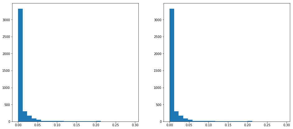
Taking a look at a distribution of the hog features showed comparable results between gray and YCrCb...this distribution was similar across various color spaces.

SVM classifier

I used the sklearn LinearSVC for training on test images. I experimented with various permutations of features, including:

HOG
HOG + spatial
HOG + color
HOG + spatial + color

At the end of all this, I was getting the best results with all features being used, HOG + spatial + color.

The function extract_features is the entry-point for extracting features for a list of images. A helper function named single_img_features can be used for testing on a single image.

To train the SVM I have a single function called train. This function uses all of the global variables defined for the various feature extraction:

color_space = 'YCrCb'
orient = 9
pix_per_cell = 8
cell_per_block = 2
hog_channel = 0
spatial_size = (32, 32)
hist_bins = 16
spatial_feat = True
hist_feat = True
hog_feat = True

Feature extraction took the majority of the time and training was fairly quick. I would routinely get above 97% accuracy:

(17760, 4884)
Using: 9 orientations 8 pixels per cell and 2 cells per block
Feature vector length: 4884
19.03 Seconds to train SVC...
Test Accuracy of SVC =  0.9789

Sliding Window Search

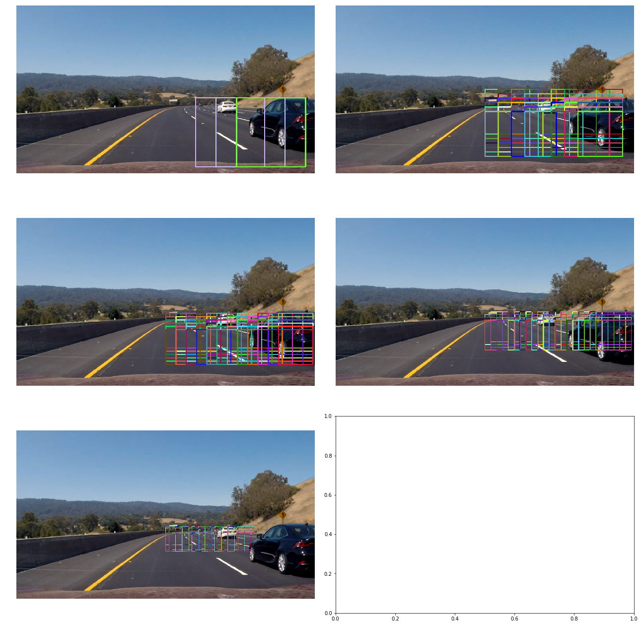
There is a single function named slide_window in cell two of the notebook which does the sliding window search. I decided upon five different categories of searches corresponding to different slices of the image:

really_close
close
medium
far
really_far

Each category consists of different parameters for the area of the image to scan, overlap and size of the box. These can all be viewed in the cell after the definition of the slide_window function.

I performed all of this imperially by:

taking a best guess
testing on sub-sampled video
making changes to the window parameters
back to 2

I found this to be a very critical part of the pipeline. Too many small areas would make the video extremely jumpy. Without enough overlap there would not be enough "hit" to identify the cars at time. Ultimately I ended up scanning with a high amount of overlap for the boxes in the mid-range size.

Below is a visualization of the final scanning regions. Boxes are drawn with random colors so it's easier to differentiate the boxes.

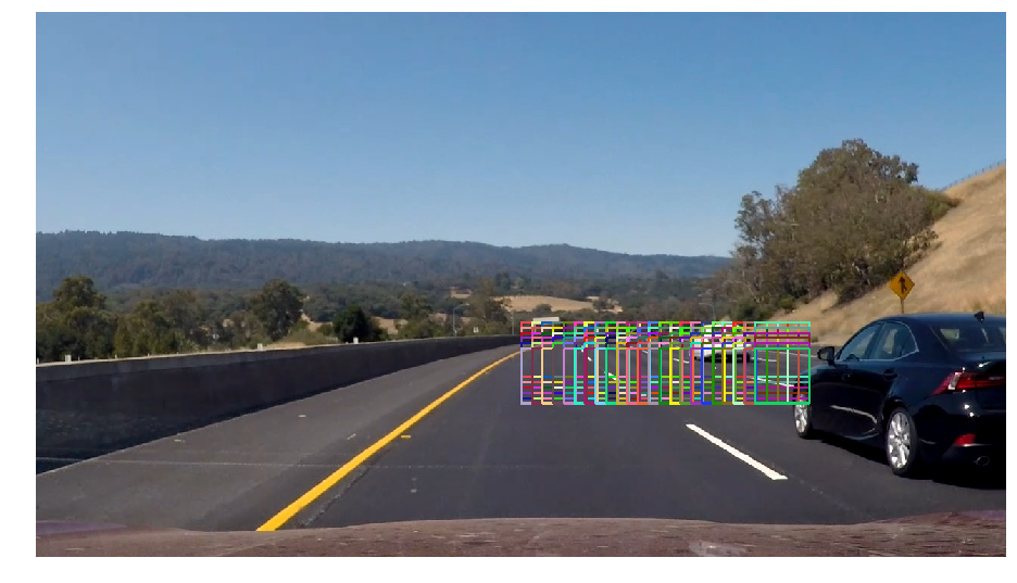
This is a larger view of the really_far scanning region:

In the pipeline I used a heatmap where every pixel contained within a bounding box was incremented by 1. Because I'm scanning with multiple sized boxes and because there is overlap a car would get "hit" by a box multiple times, typically. From time to time there would be a false-positive in a random location. The heatmap would produce an image which would get brighter as there were more "hits".

I applied a threshold of 3 to keep any regions meaning there had to be at least three "hits" on an area in order for it to be kept.

Once the thresholding was applied I used the label function from scipy to determine the final areas of interest and the bounding boxes for the final boxes.

Here are a few frames and their corresponding heatmaps. In all images below the first column displays all of the detected car images or "hits" for a particular box during the sliding window:

Here is the output of scipy.ndimage.measurements.label() on the integrated heatmap:

Below are some examples of the final results...all of the boxes are drawn in the first column while the second column consists of the "final" boxes after heatmap and thresholding:

Discussion

I found that it was critical to get the right number and size of scanning windows. I went through various permutations and had choppy videos at the beginning due to too many small windows. After a few iterations I found better results by doing many overlapping scans in the mid-range of the box sizes.

As seen in the example sliding windows, I scan from the left to the right which ends up stopping short of the right edge of the frame. This results in the cars not being detected until they are in clear view. It could help to add some additional scanning from the right to the left.

brianz / udacity-sdc-p5