Fast Normal CDF

Introduction

The standard normal CDF $\Phi(x)$ is an important function in a broad range of statistical problems. When we need to evaluate the function many times (for example in numerical integration), the computation performance may become an issue.

One way to fast evaluate the function is to use a look-up table, that is, we pre-compute a set of pairs $(x_i, \Phi(x_i))$ ` and then use interpolation to approximate the function value of a given .

This simple library calculates the $\Phi(x)$ function using piecewise linear interpolation. The approximation error is guaranteed to be no greater than $\epsilon = 10^{-7}$ .

Installation

The package can be installed from Github by calling:

remotes::install_github("boennecd/fastncdf")

Algorithm

We need to first determine the knots that we want to pre-compute. Since $\Phi(-x) = 1 - \Phi(x)$ , we only need to consider non-negative ’s.

For $x > \Phi^{-1}(1 - \epsilon) = 5.1993376$ , we set $\Phi(x) = 1$ and hence the error is bounded by $\epsilon$ . Let , , , where is the smallest integer such that . Then we need to determine the interval width to satisfy the error bound.

For piecewise linear interpolation, the error is bounded by

$E(t) \leq 1/8 \cdot \lVert f''\rVert_{\infty}h^2$

(Source http://pages.cs.wisc.edu/~amos/412/lecture-notes/lecture09.pdf)

Since $\Phi''(x) = \phi'(x) = -x \phi(x)$ , it can be shown that $\lVert \Phi''\rVert_\infty = \psi(1) = 0.2419707$ .

Therefore, can be calculated as:

(h <- sqrt(8 / dnorm(1) * 1e-7))

## [1] 0.001818292

So the s and s values are:

x <- seq(0, qnorm(1 - 1e-7) + h, by = h)
length(x)

## [1] 2861

y <- pnorm(x)

We can then call dput(x) and dput(y) to get the data we need.

Performance

We compare the speed of fastpnorm() and fastpnorm_preallocated() with pnorm() in R:

library(fastncdf)
u <- seq(-6, 6, by = 1e-6)
system.time(truth <- pnorm(u))

##    user  system elapsed 
##   0.487   0.028   0.516

system.time(fasty <- fastpnorm(u))

##    user  system elapsed 
##   0.041   0.020   0.060

system.time(fasty_prec <- fastpnorm(u, TRUE))

##    user  system elapsed 
##   0.130   0.016   0.146

range(truth - fasty)

## [1] -9.99999e-08  9.99999e-08

range(truth - fasty_prec)

## [1] -9.99999e-08  9.99999e-08

# if we already had a vector with values then we can use a faster version
res <- rep(0., length(u))
system.time(fastpnorm_preallocated(u, res))

##    user  system elapsed 
##    0.03    0.00    0.03

all.equal(res, fasty)

## [1] TRUE

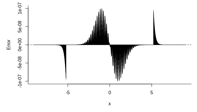
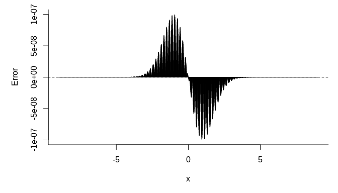
We plot the error versus the quantile below:

par(mar = c(5, 5, 1, 1))
us <- seq(-9, 9, length.out = 2000)
plot(us, fastpnorm(us) - pnorm(us), type = "h",
     bty = "l", xlab = expression(x), ylab = "Error")
abline(h = 0, lty = 2)

plot(us, fastpnorm(us, TRUE) - pnorm(us), type = "h",
     bty = "l", xlab = expression(x), ylab = "Error")
abline(h = 0, lty = 2)

Other Interpolation Methods

We can get a similar result using R’s approxfun to do linear interpolation:

lin_aprx <- local({
  f <- approxfun(x = x, y = y, yleft = 0.5, yright = 1)
  function(x){
    p <- f(abs(x))
    ifelse(x < 0, 1 - p, p)
  }
})

max(abs(lin_aprx(u) - fastpnorm(u)))

## [1] 1.554312e-15

The R version is slower though:

system.time(lin_aprx(u))

##    user  system elapsed 
##   0.475   0.156   0.631

system.time(fastpnorm(u))

##    user  system elapsed 
##   0.032   0.028   0.060

We can though use R’s splinefun to see the performance of other functions. In particular, we can consider monotone cubic interpolation using Fritsch–Carlson method:

m_splin <- local({
  n_points <- 300L
  eps <- 1e-9
  x <- seq(0, qnorm(1 - eps), length.out = n_points)
  f <- splinefun(x = x, y = pnorm(x), method = "monoH.FC")
  x_max <- max(x)
  
  function(x){
    p <- f(abs(x))
    out <- ifelse(x < 0, 1 - p, p)
    ifelse(abs(x) > x_max, .5 * (1 + sign(x)), out)
  }
})

# check the error 
range(truth - m_splin(u))

## [1] -5.165321e-08  5.165321e-08

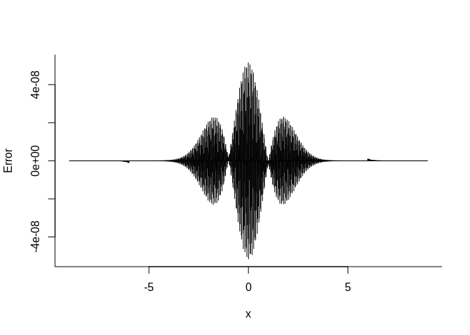
# plot the error
plot(us, m_splin(us) - pnorm(us), type = "h",
     bty = "l", xlab = expression(x), ylab = "Error")

We will require three doubles per knot unlike the two we need for the linear interpolation. Furthermore, more computation is needed to perform the interpolation. However, we may need much fewer knots as shown above and this will reduce the cache misses.

A C++ implementation is also provided with this package:

all.equal(m_splin(u), fastpnorm(u, use_cubic = TRUE))

## [1] TRUE

system.time(aprx_cubic <- fastpnorm(u, use_cubic = TRUE))

##    user  system elapsed 
##   0.076   0.024   0.101

max(abs(aprx_cubic - truth))

## [1] 5.165321e-08

res <- rep(0., length(u))
system.time(fastpnorm_preallocated(u, res, use_cubic = TRUE))

##    user  system elapsed 
##   0.073   0.000   0.073

all.equal(res, aprx_cubic)

## [1] TRUE

We can compare the monotone cubic interpolation with the linear interpolation with a particular focus on how well they scale in the number of threads used in the computation:

res <- rep(0, length(u))
test_func <- function(use_cubic, n_threads)
  fastpnorm_preallocated(u, res, n_threads = n_threads, 
                         use_cubic = use_cubic)

bench::mark(
  `pnorm             ` = pnorm(u),
  `linear (1 thread) ` = test_func(FALSE, 1L),
  `linear (2 threads)` = test_func(FALSE, 2L),
  `linear (4 threads)` = test_func(FALSE, 4L),
  `linear (6 threads)` = test_func(FALSE, 6L),
  `cubic  (1 thread) ` = test_func(TRUE , 1L),
  `cubic  (2 threads)` = test_func(TRUE , 2L),
  `cubic  (4 threads)` = test_func(TRUE , 4L),
  `cubic  (6 threads)` = test_func(TRUE , 6L),
  check = FALSE, min_time = 2)

## # A tibble: 9 x 6
##   expression              min   median `itr/sec` mem_alloc `gc/sec`
##   <bch:expr>         <bch:tm> <bch:tm>     <dbl> <bch:byt>    <dbl>
## 1 pnorm               508.7ms  519.2ms      1.92    91.6MB        0
## 2 linear (1 thread)    29.2ms   30.3ms     32.8         0B        0
## 3 linear (2 threads)     18ms     19ms     51.7    668.5KB        0
## 4 linear (4 threads)   17.7ms     19ms     52.1         0B        0
## 5 linear (6 threads)   17.9ms   18.9ms     51.6         0B        0
## 6 cubic  (1 thread)    68.9ms   69.6ms     14.2         0B        0
## 7 cubic  (2 threads)   35.3ms   35.7ms     27.5         0B        0
## 8 cubic  (4 threads)   18.7ms   20.2ms     49.0         0B        0
## 9 cubic  (6 threads)   18.2ms     19ms     52.0         0B        0

We may prefer the monotone cubic interpolation given the lower error, lower memory requirements, it scales better in the number of threads, and it has less “sided” errors.

boennecd / fastncdf