Cartographic rendering and mesh analytics powered by PyVista
| ⚙️ CI | |
| 💬 Community |   |
| 📚 Docs | |
| 📈 Health | |
| ✨ Meta |   |
| 📦 Package |    |
| 🧰 Repo |    |
| 🛡️ Status | |
smc-timeseries.mov
GeoVista is built on the shoulders of giants, namely PyVista and VTK, thus allowing it to easily leverage the power of the GPU.
As a result, it offers a paradigm shift in rendering performance and interactive user experience, as demonstrated by this realtime, time-series animation of WAVEWATCH III® third-generation wave model (WAVE-height, WATer depth and Current Hindcasting) data developed at NOAA/NCEP.
The animation shows a time-series of Sea Surface Wave Significant Height data located on the cell faces of a quasi-unstructured Spherical Multi-Cell (SMC) grid.
Bring your data alive with GeoVista! 🚀
Keen to know more? Well, let's begin ...
The goal of GeoVista is simple; to complement PyVista with a convenient cartographic capability.
In this regard, from a design perspective we aim to keep GeoVista as pure to PyVista as possible i.e., minimise specialisation as far as practically possible in order to maximise native compatibility within the PyVista and VTK ecosystems.
We intend GeoVista to be a cartographic gateway into the powerful world of PyVista, and all that it offers.
GeoVista is intentionally agnostic to packages such as geopandas, iris, xarray et al, which specialise in preparing your spatial data for visualisation. Rather, we delegate that responsibility and choice of tool to you the user, as we want GeoVista to remain as flexible and open-ended as possible to the entire Scientific Python community.
Simply put, "GeoVista is to PyVista", as "Cartopy is to Matplotlib". Well, that's the aspiration.
GeoVista is available on both conda-forge and PyPI.
We recommend using conda to install GeoVista 👍
GeoVista is available on conda-forge, and can be easily installed with conda:
conda install -c conda-forge geovistaFor more information see our conda-forge feedstock and prefix.dev dashboard.
GeoVista is also available on PyPI:
pip install geovistaCheckout out our PyPI Download Stats, if you like that kinda thing.
If you simply can't wait for the next release to play with the latest hot features, then you can easily
install the main development branch from GitHub:
pip install git+https://github.com/bjlittle/geovista@mainAlternatively, to configure a full developer environment, first clone the GeoVista GitHub repository:
git clone git@github.com:bjlittle/geovista.gitChange to the root directory:
cd geovistaCreate the geovista-dev conda development environment:
conda env create --file requirements/geovista.ymlNow activate the environment and install the main development branch of GeoVista:
conda activate geovista-dev
pip install --no-deps --editable .
Finally, you're good to roll 🥳
And for extra credit, install our developer pre-commit git-hooks:
pre-commit installGeoVista comes with various pre-canned resources to help get you started on your visualisation journey.
GeoVista makes use of various resources, such as rasters, VTK meshes, Natural Earth features, and sample model data.
If you want to download and cache all registered GeoVista resources to make them available offline, simply:
geovista download --allAlternatively, just leave GeoVista to download resources on-the-fly, as and when she needs them.
To view the list of registered resources, simply:
geovista download --listWant to know more?
geovista download --helpLet's explore a sample of various oceanographic and atmospheric model data using GeoVista.
First, let's render a WAVEWATCH III (WW3) unstructured triangular mesh, with 10m Natural Earth coastlines, a 1:50m Natural Earth Cross-Blended Hypsometric Tints base layer, and the gorgeous perceptually uniform cmocean balance diverging colormap.
🗒 click for code
import geovista as gv
from geovista.pantry import ww3_global_tri
import geovista.theme

# Load the sample data.
sample = ww3_global_tri()

# Create the mesh from the sample data.
mesh = gv.Transform.from_unstructured(
    sample.lons, sample.lats, connectivity=sample.connectivity, data=sample.data
)

# Plot the mesh.
plotter = gv.GeoPlotter()
sargs = {"title": f"{sample.name} / {sample.units}"}
plotter.add_mesh(mesh, show_edges=True, scalar_bar_args=sargs)
plotter.add_base_layer(texture=gv.natural_earth_hypsometric())
plotter.add_coastlines()
plotter.add_graticule()
plotter.view_xy(negative=True)
plotter.add_axes()
plotter.show()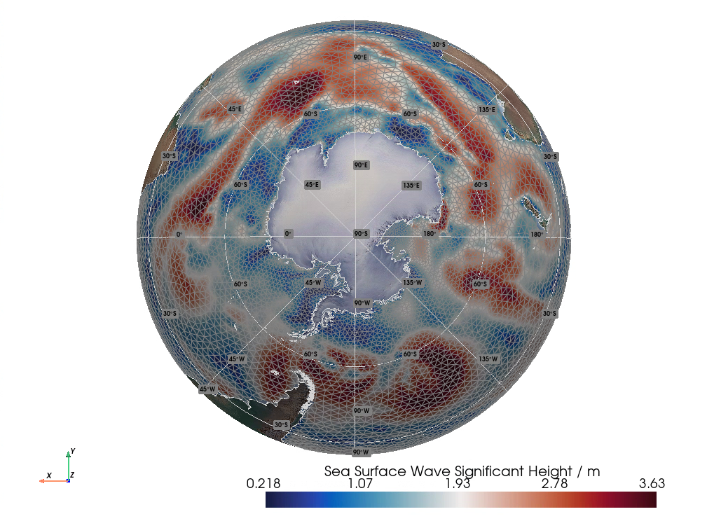
Now, let's visualise the bathymetry of the Plymouth Sound and Tamar River from an FVCOM unstructured mesh, as kindly provided by the Plymouth Marine Laboratory using the lush cmocean deep colormap.
🗒 click for code
import geovista as gv
from geovista.pantry import fvcom_tamar
import geovista.theme

# Load the sample data.
sample = fvcom_tamar()

# Create the mesh from the sample data.
mesh = gv.Transform.from_unstructured(
    sample.lons,
    sample.lats,
    connectivity=sample.connectivity,
    data=sample.face,
    name="face",
)

# Warp the mesh nodes by the bathymetry.
mesh.point_data["node"] = sample.node
mesh.compute_normals(cell_normals=False, point_normals=True, inplace=True)
mesh.warp_by_scalar(scalars="node", inplace=True, factor=2e-5)

# Plot the mesh.
plotter = gv.GeoPlotter()
sargs = {"title": f"{sample.name} / {sample.units}"}
plotter.add_mesh(mesh, cmap="deep", scalar_bar_args=sargs)
plotter.add_axes()
plotter.show()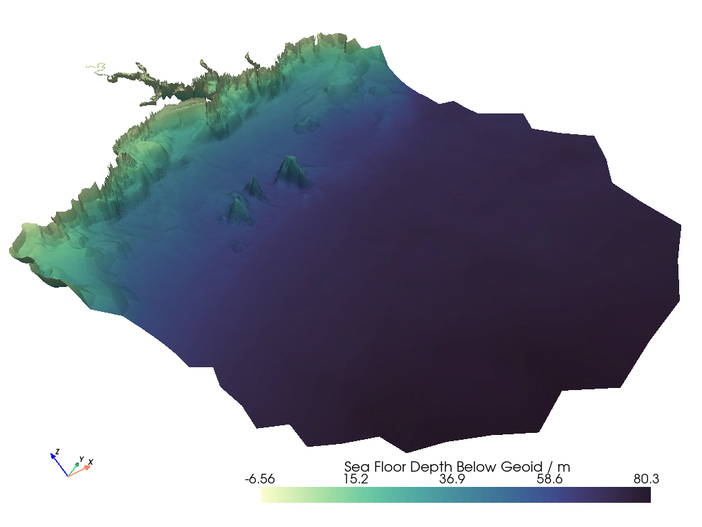
Initial projection support is available within GeoVista for Cylindrical and Pseudo-Cylindrical projections. As GeoVista matures and stabilises, we'll aim to complement this capability with other classes of projections, such as Azimuthal and Conic.
In the meantime, let's showcase our basic projection support with some high-resolution unstructured Local Area Model (LAM) data reprojected to Mollweide using a PROJ string, with 10m Natural Earth coastlines and a 1:50m Natural Earth Cross-Blended Hypsometric Tints base layer.
🗒 click for code
import geovista as gv
from geovista.pantry import lam_pacific
import geovista.theme

# Load the sample data.
sample = lam_pacific()

# Create the mesh from the sample data.
mesh = gv.Transform.from_unstructured(
    sample.lons,
    sample.lats,
    connectivity=sample.connectivity,
    data=sample.data,
)

# Plot the mesh on a mollweide projection using a Proj string.
plotter = gv.GeoPlotter(crs="+proj=moll")
sargs = {"title": f"{sample.name} / {sample.units}"}
plotter.add_mesh(mesh, scalar_bar_args=sargs)
plotter.add_base_layer(texture=gv.natural_earth_hypsometric())
plotter.add_coastlines()
plotter.add_graticule()
plotter.add_axes()
plotter.view_xy()
plotter.show()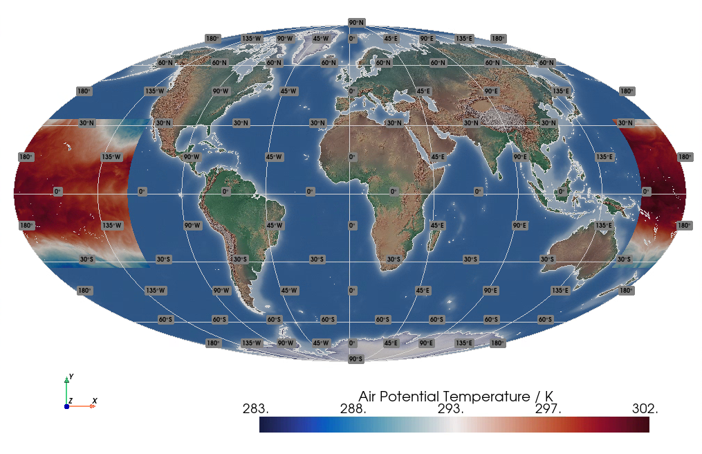
Using the same unstructured LAM data, reproject to Equidistant Cylindrical but this time using a Cartopy Plate Carrée CRS, also with 10m Natural Earth coastlines and a 1:50m Natural Earth Cross-Blended Hypsometric Tints base layer.
🗒 click for code
import cartopy.crs as ccrs

import geovista as gv
from geovista.pantry import lam_pacific
import geovista.theme

# Load the sample data.
sample = lam_pacific()

# Create the mesh from the sample data.
mesh = gv.Transform.from_unstructured(
    sample.lons,
    sample.lats,
    connectivity=sample.connectivity,
    data=sample.data,
)

# Plot the mesh on a Plate Carrée projection using a cartopy CRS.
plotter = gv.GeoPlotter(crs=ccrs.PlateCarree(central_longitude=180))
sargs = {"title": f"{sample.name} / {sample.units}"}
plotter.add_mesh(mesh, scalar_bar_args=sargs)
plotter.add_base_layer(texture=gv.natural_earth_hypsometric())
plotter.add_coastlines()
plotter.add_graticule()
plotter.add_axes()
plotter.view_xy()
plotter.show()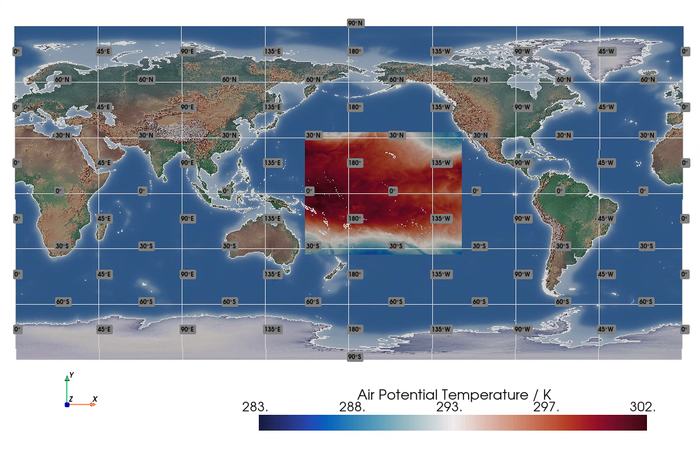
Now render a Met Office LFRic C48 cube-sphere unstructured mesh of Sea Surface Temperature data on a Robinson projection using an ESRI SRID, with 10m Natural Earth coastlines and a cmocean thermal colormap.
🗒 click for code
import geovista as gv
from geovista.pantry import lfric_sst
import geovista.theme

# Load the sample data.
sample = lfric_sst()

# Create the mesh from the sample data.
mesh = gv.Transform.from_unstructured(
    sample.lons,
    sample.lats,
    connectivity=sample.connectivity,
    data=sample.data,
)

# Plot the mesh on a Robinson projection using an ESRI spatial reference identifier.
plotter = gv.GeoPlotter(crs="ESRI:54030")
sargs = {"title": f"{sample.name} / {sample.units}"}
plotter.add_mesh(mesh, cmap="thermal", show_edges=True, scalar_bar_args=sargs)
plotter.add_coastlines()
plotter.view_xy()
plotter.add_axes()
plotter.show()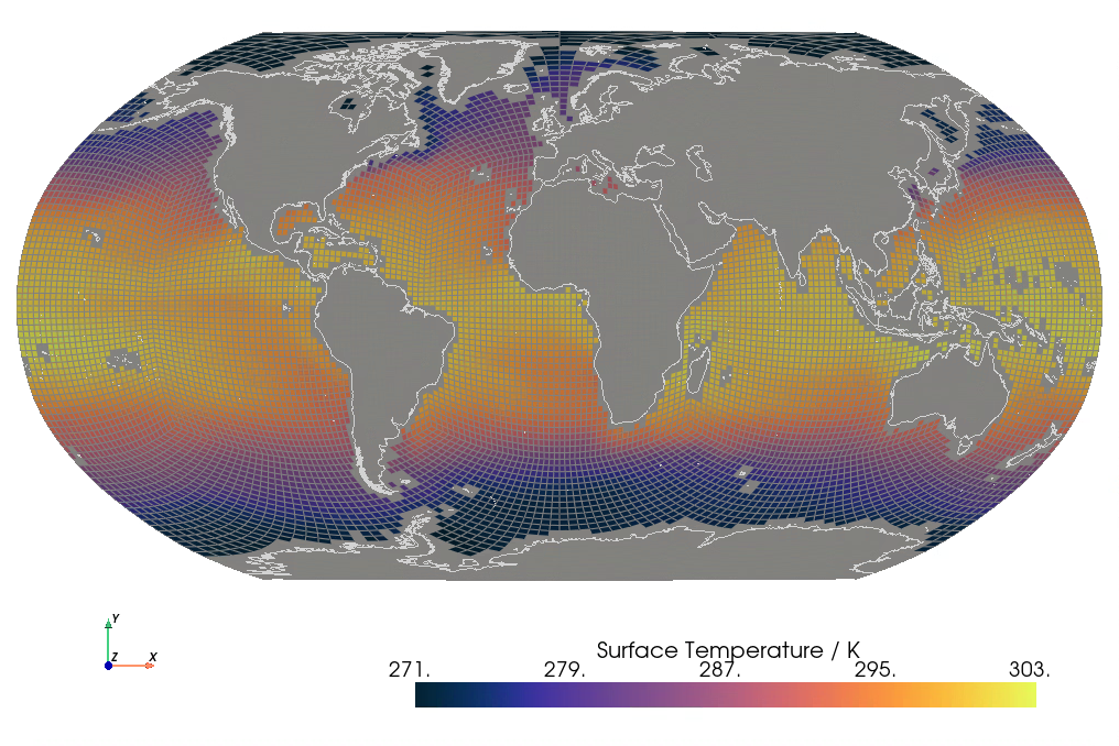
So far we've demonstrated GeoVista's ability to cope with unstructured data. Now let's plot a curvilinear mesh using Nucleus for European Modelling of the Ocean (NEMO) ORCA2 Sea Water Potential Temperature data, with 10m Natural Earth coastlines and a 1:50m Natural Earth I base layer.
🗒 click for code
import geovista as gv
from geovista.pantry import nemo_orca2
import geovista.theme

# Load sample data.
sample = nemo_orca2()

# Create the mesh from the sample data.
mesh = gv.Transform.from_2d(sample.lons, sample.lats, data=sample.data)

# Remove cells from the mesh with NaN values.
mesh = mesh.threshold()

# Plot the mesh.
plotter = gv.GeoPlotter()
sargs = {"title": f"{sample.name} / {sample.units}"}
plotter.add_mesh(mesh, show_edges=True, scalar_bar_args=sargs)
plotter.add_base_layer(texture=gv.natural_earth_1())
plotter.add_coastlines()
plotter.view_xy()
plotter.add_axes()
plotter.show()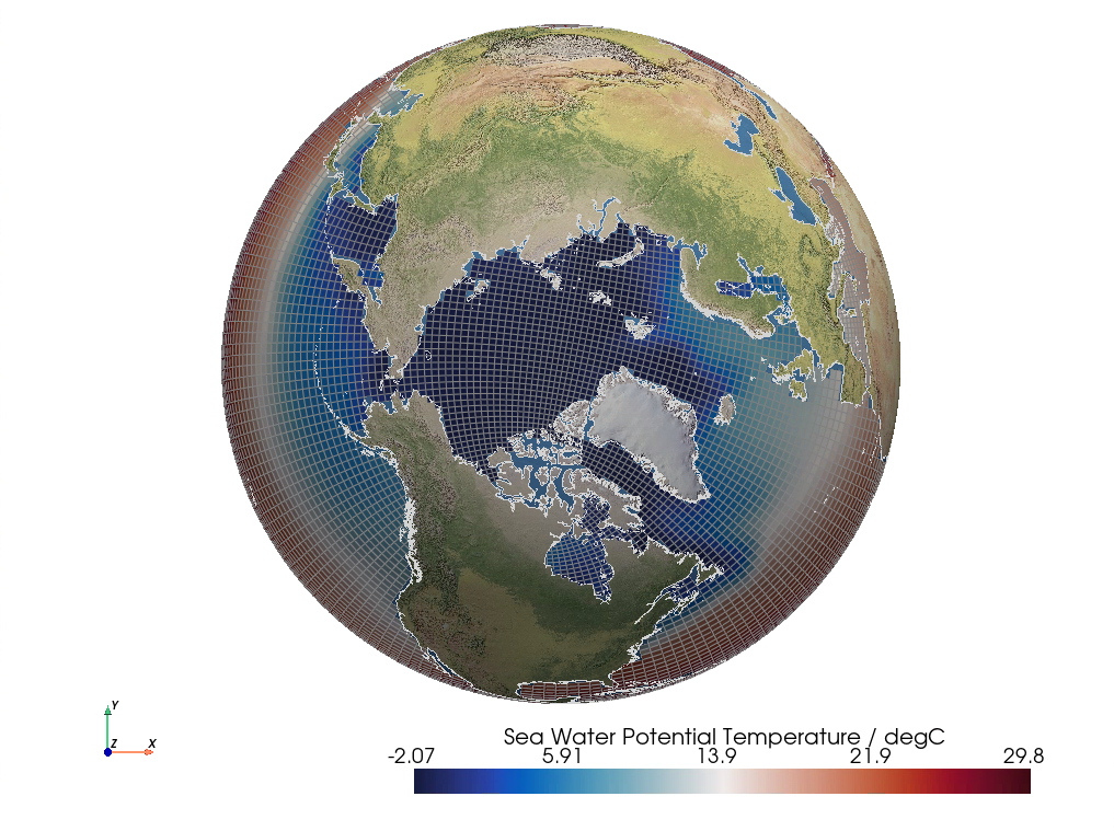
Now let's render a NOAA/NCEI Optimum Interpolation SST (OISST) Advanced Very High Resolution Radiometer (AVHRR) rectilinear mesh, with 10m Natural Earth coastlines and a NASA Blue Marble base layer.
🗒 click for code
import geovista as gv
from geovista.pantry import oisst_avhrr_sst
import geovista.theme

# Load sample data.
sample = oisst_avhrr_sst()

# Create the mesh from the sample data.
mesh = gv.Transform.from_1d(sample.lons, sample.lats, data=sample.data)

# Remove cells from the mesh with NaN values.
mesh = mesh.threshold()

# Plot the mesh.
plotter = gv.GeoPlotter()
sargs = {"title": f"{sample.name} / {sample.units}"}
plotter.add_mesh(mesh, scalar_bar_args=sargs)
plotter.add_base_layer(texture=gv.blue_marble())
plotter.add_coastlines()
plotter.view_xz()
plotter.add_axes()
plotter.show()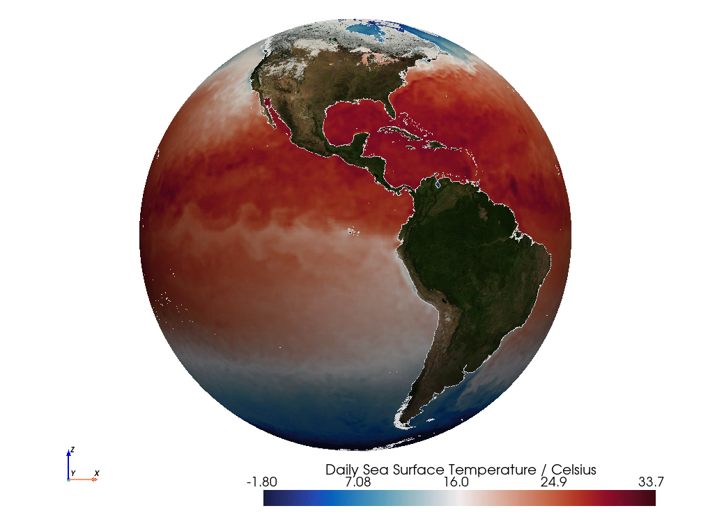
Finally, to demonstrate support for non-traditional cell geometries i.e., not triangles or quadrilaterals, we plot the unstructured mesh from the DYNAMICO project. This model uses hexagonal and pentagonal cells, and is a new dynamical core for LMD-Z, the atmospheric General Circulation Model (GCM) part of the IPSL-CM Earth System Model. The render also contains 10m Natural Earth coastlines.
🗒 click for code
import geovista as gv
from geovista.pantry import dynamico
import geovista.theme

# Load sample data.
sample = dynamico()

# Create the mesh from the sample data.
mesh = gv.Transform.from_unstructured(sample.lons, sample.lats, data=sample.data)

# Plot the mesh.
plotter = gv.GeoPlotter()
sargs = {"title": f"{sample.name} / {sample.units}"}
plotter.add_mesh(mesh, scalar_bar_args=sargs)
plotter.add_coastlines()
plotter.add_axes()
plotter.show()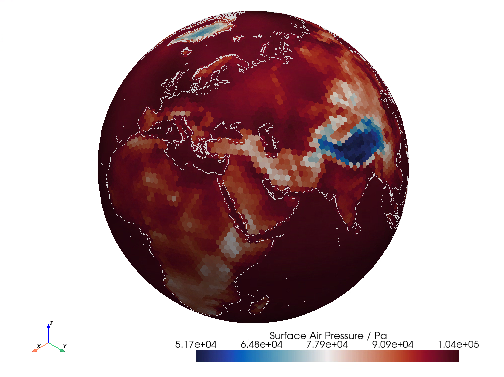
"Please, sir, I want some more", Charles Dickens, Oliver Twist, 1838.
Certainly, our pleasure! From the command line, simply:
geovista examples --run all --verboseWant to know more?
geovista examples --helpThe documentation is built by Sphinx and hosted on Read the Docs.
Whilst you're here, why not hop on over to the pyvista-xarray project and check it out!
It's aiming to provide xarray DataArray accessors for PyVista to visualize datasets in 3D for the
xarray community, and will be building on top of GeoVista 🎉
Need help? 😢
Why not check out our existing GitHub issues. See something similar? Well, give it a 👍 to raise its priority and feel free to chip in on the conversation. Otherwise, don't hesitate to create a new GitHub issue instead.
However, if you'd rather have a natter, then head on over to our GitHub Discussions. That's definitely the place to wax lyrical all things GeoVista!
GeoVista is distributed under the terms of the BSD-3-Clause license.

Graphics and Lead Scientist: Ed Hawkins, National Centre for Atmospheric Science, University of Reading.
Data: Berkeley Earth, NOAA, UK Met Office, MeteoSwiss, DWD, SMHI, UoR, Meteo France & ZAMG.
#ShowYourStripes is distributed under a
Creative Commons Attribution 4.0 International License
