README

#Spark #R #iGraph

Background

Instacart, an American company who provides groceries delivery service releases their shopping dataset publicly. This anonymized dataset contains a sample of over 3 million grocery orders from more than 200,000 Instacart users. Over here, we will simply do a data exploratory using association rule and graph techniques.

Import Data to Spark

To facilitate the data processing (~ 500MB), we run a local Spark cluster on our machine through SparklyR.

library(sparklyr)
library(dplyr)
library(readr)
library(purrr)
library(igraph)
library(visNetwork)

# Spark properties
conf <- spark_config()
conf$`sparklyr.cores.local` <- 4
conf$`sparklyr.shell.driver-memory` <- "8G"
conf$`spark.memory.fraction` <- 0.9
sc <- spark_connect(master = "local", version = "2.2.0", config = conf)

Frequent Pattern Mining

With Spark activated, we read our data into a Spark dataframe. Spark has built-in FP Growth algorithm implementation. All we need to specify hyperparameters mininum confidence and mininum support. For more about the algorithm, see here.

Note: You need at least SparklyR version 2.2.0 for FP Growth algorithm implementation.

# this is our data from Instacart
orders <- spark_read_csv(sc, "orders", "instacart_2017_05_01/order_products__prior.csv")
# group items by order (purchase history)
orders_wide <- orders %>% 
    group_by(order_id) %>% 
    summarise(items = collect_list(product_id))

# invoke FP Growth implementation
fpg.fit <- ml_fpgrowth(orders_wide, items_col = "items", min_confidence = .015, min_support = .005)
rules <- ml_association_rules(fpg.fit) %>% collect()

This is basically it. We have a list showing which item is associated with what, as in {antecedent}--{consequent}.

# collect our rules into a data frame
asso <-
    tibble(
        antecedent = unlist(rules$antecedent),
        consequent = unlist(rules$consequent),
        confidence = rules$confidence
    )
head(asso)

## # A tibble: 6 x 3
##   antecedent consequent confidence
##        <int>      <int>      <dbl>
## 1       4605      24852      0.289
## 2      26209      21137      0.135
## 3      26209      47766      0.157
## 4      26209      47209      0.142
## 5      26209      13176      0.148
## 6      26209      21903      0.148

# remember to close Spark connection
spark_disconnect_all()

## [1] 1

Visualizing Result

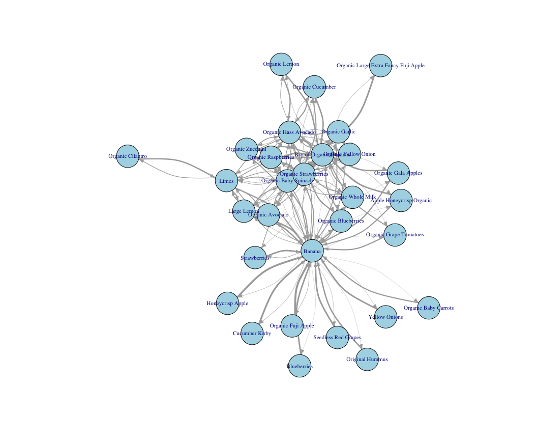
Fundamentally, what we have done so far is to create a network of ‘food’, {A}--{B} and {B}--{C} and etc. We will proceed to visualize it using igraph library. Please note that the width of edge or relationship between nodes signifies the confidence. With food {A} usually associates with food {B}, the other way around may not be true. If someone bought a salmon, he or she may also buy a lemon. For someone who buys lemon, to buy salmon as well may not be necessary.

# get product names
products <- read_csv("instacart_2017_05_01/products.csv")

# bind to nodes
nodes <- data.frame(id = unique(asso$antecedent, asso$consequent)) %>% 
    distinct() %>% 
    left_join(products, by = c("id" = "product_id")) %>% 
    select(id, label = product_name)

edges <- asso %>% mutate(weight = confidence * 10)

df.g <- graph_from_data_frame(edges, directed = TRUE, vertices = nodes)
plot(
    df.g,
    edge.arrow.size = .5,
    edge.curved = .3,
    edge.width = edges$weight,
    vertex.color = "lightblue",
    vertex.label.color = "darkblue",
    vertex.label.cex = .7,
    edge.label.cex = .7
)

Another way of visualizing the network is through interactive plotting library VisNetwork. The code is shown below but the result won’t be displayed in static HTML here.

nodes <- data.frame(id = unique(asso$antecedent, asso$consequent)) %>% 
    distinct() %>% 
    left_join(products, by = c("id" = "product_id")) %>% 
    select(id, label = product_name)

edges <- asso %>% 
    mutate(width = confidence * 20, 
           smooth = TRUE, arrows = "to",
           label = format(confidence, digits = 2)) %>% 
    rename(from = antecedent, to = consequent)

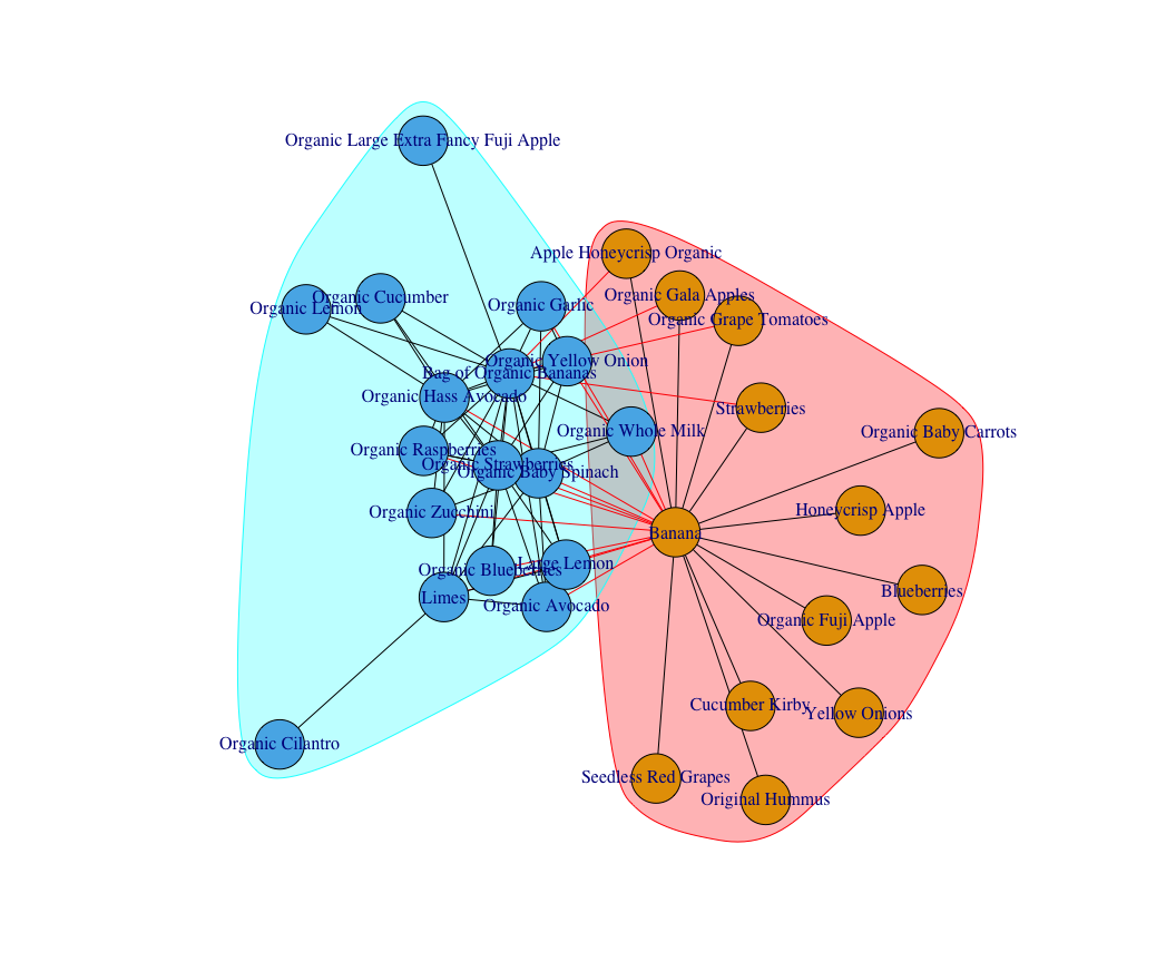
visNetwork(nodes, edges, height = "800px", width = "100%")

Cluster Detection

With a graph in place, it is easy to proceed with more interesting discovery. With merely two lines of code, we can cluster items using graph community detection technique. Awesome.

# community structure detection requires no directed graph
df.g.sym <- as.undirected(df.g, mode = "collapse", edge.attr.comb = list(weight = "sum", "ignore"))
ceb <- cluster_edge_betweenness(df.g.sym)
#dendPlot(ceb, mode = "hclust")
plot(ceb, df.g.sym)

Data Source

“The Instacart Online Grocery Shopping Dataset 2017”, Accessed from https://www.instacart.com/datasets/grocery-shopping-2017 on 2019-05-22.

bj-sodas / online-retail