With this project, I aimed at analyzing a neural network from the ground up that could classify handwritten numbers. The MNIST data set is a common starting place for many machine learning approaches and its large data set proved ideal for building my network. The program is written in Python 2.7 and the MNIST data can be found here: http://yann.lecun.com/exdb/mnist/
Before looking at the code, it is important to understand what a neural network is and how it functions. A neural network is an “information processing paradigm” that uses a system of neurons, configured in layers, to make decisions. This network is dependent on two important players: the weights and biases that guide the decision making of each neuron. Using these weights and biases, neurons are able to take binary input, pass judgement according to those parameters, and create an output. Next, a learning algorithm tunes the weights and biases of each neuron so the network as a whole can properly evaluate inputs to achieve the correct output.

The decision making machine that is the neural network starts with the smallest component: the neuron. There are many options for neurons, the most basic being the perceptron, however for my purposes the sigmoid neuron was ideal. The sigmoid neuron, unlike the perceptron, takes input values from 0 to 1 and determines output according to the following equation - the ‘sigmoid function’:
σ(z)≡1/(1+e^-z)
Where z = w⋅x+b
This function evaluates the array of inputs, x, and multiplies them by how important each input is, or the weight, w. Next it adds the bias, b, which acts as a threshold to the neuron. This results in a value z, which is essential to the sigmoid equation. If z is a large positive value then e^-z≈0 and so σ(z)≈1, which is the output of the neuron. On the contrary if z is a large negative value then e^-z≈∞ and so σ(z)≈0. The most important takeaway from this function is that it is able to output any value between 0 and 1, and that small changes in weights and biases only produce a small change in output. This is unlike the perceptron neuron, which only outputs 0 or 1, and is too responsive to minor changes in weights and biases. The sigmoid neurons ability to take inputs and evaluate them according to weights and biases that can be easily adjusted make it ideal to be the main component of the neural network.
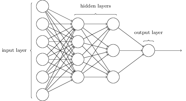
Now that the use of sigmoid neurons is clear it is important to document how they will be used to form a network. This neural network will have three layers: an input layer, a single hidden layer, and an output layer. The input layer, in this case, will encode the thousands of images of handwritten numbers and evaluate each pixel. Each MNIST image is a 28 x 28 gray scale image, therefore it is necessary to have 784 input neurons to evaluate each pixel (0 is black, 1.0 is white with grey in between). After the pixels are evaluated by the input layer, each input neuron passes its output to the hidden layer, which can have a variable amount of neurons. The more neurons the hidden layer has the more accurate the network will be, to a point. Each hidden neuron will evaluate a variable amount of the data from the input layer and all the hidden layers together will have evaluated each pixel. The output layer has 10 neurons, each corresponding to a number 0 to 9, and the neuron with the highest activation value will be the number the network guesses the handwritten digit is.
After understanding what a network of neurons looks like, it is important to understand how a network can learn. The learning process consists of tuning the weights and biases of each neuron, using the training set of data from MNIST, in order to find a configuration that returns the most accurate results when evaluating the images of handwritten digits. The learning process starts with a cost function, an algorithm that shows how accurate the decision of the network is versus the actual number value of an image. If the output of the network is a 10 - dimensional vector generated from the network evaluating inputs then if the network guessed ‘6’, the output would be y(x) = (0, 0, 0, 0, 0, 0, 1, 0, 0, 0) ideally. The cost function is as follows:
Here cost, C, is a function dependent on the weights and biases of the network, w and b. The total number of training inputs is n, y(x) represents the prediction of the network and a represents the vector of outputs containing the correct value from the training data set. This resulting quadratic function is non-negative, as every term is positive, and that it is a great indication of how accurate the network is. If the output of the network (y(x)) is very close to the actual value (a) then C(w,b)≈0, and if C(w,b) is large then the output of the network is not close to the value of the image, it is inaccurate. The cost function is important because in order to increase the accuracy of the network, it is necessary to reduce and minimize the cost of the cost function. In conclusion, the goal is to train a neural network that finds weights and biases that minimizes C(w,b), which in turn would be a network that could accurately predict the true values of handwritten images.
The goal now is to minimize the cost function. If the cost function was for a network with just one input variable, then simple calculus would find the combination of weights and biases that minimize the function. However that is not the case here, and instead the cost function has many inputs from hundreds of neurons, and in order to minimize this function the technique of gradient descent must be used. This was a difficult topic for me to grasp and I recommend reading Michael Nielson’s explanation in his textbook. With that said, gradient descent is a technique to minimize a multivariable function using an iterative optimization algorithm. A graph with many variables that are all quadratic in nature, due to the nature of the cost function, is characterized by a gradient (∇C, a generalization of the multi-variable derivative, which is not a scalar but instead a vector). ΔC≈∇C⋅Δv is essentially the equation that needs to be minimized, this is done by using small intervals (in this example Δv would be a small fixed value, or ‘step) to move through the graph. Nielson sums up gradient descent as “a way of taking small steps in the direction which does the most to immediately decrease C” as a way to reach the minimum.
In order to find the minimum of this multi-dimensional function it is necessary to ‘update’ each of the input variables by a small amount, resulting in a new Cost value that is closer to the minimum. The updated functions for weights and biases are as follows:
It is important to note that this equation is finding the weights and biases that minimize the cost function. The function works essentially by taking small steps based on η, or the learning rate, down the slope of Cost (taking the partial derivative of Cost) until a minimum is reached.
This method is adapted to assist in computing time by only applying gradient descent to a small group of images or inputs, this is known as stochastic gradient descent.
The entire project is contained in two python files. The mnist_loader is a library used to parse the training and test date from the data folder. The network file contains a network object that will represent the entire neural network. In order to run the network first load the training, validation and test data from mnist_loader. In a python shell:
import mnist_loader
training_data, validation_data, test_data = \
... mnist_loader.load_data_wrapper()
Next initialize an instance of the network. The network takes 3 paramaters for 3 layers of the nerual network. The first layer is 784 neurons, the hidden layer is a variable amount, in this example 40 neurons, and the output layer has 10 neurons.
import network
net = network.Network([784, 40, 10])
Now to start the learning process use the stochastic gradient descent method from the network instance. Note important parameters like the number of epochs or cycles, the mini-batch size, and the learning rate.
net.SGD(training_data, 30, 10, 3.0, test_data=test_data)
Benjamin Hughes
This project is licensed under the MIT License - see the LICENSE.md file for details
This would not be possible without the detailed instruction of Michael Nielsen in Neural Networks and Deep Learning. Found at: http://neuralnetworksanddeeplearning.com