The ESDist package is designed to calculate and visualise
field-specific effect size distributions, based on data that can easily
be obtained from meta-analyses.
You can install the ESDist package from GitHub
with:
library(devtools)
devtools::install_github("berntgl/ESDist")
#> stringi (1.8.3 -> 1.8.4) [CRAN]
#>
#> The downloaded binary packages are in
#>  /var/folders/j7/lmhpj_jj73qfc31klr2wh3vw0000gp/T//RtmprxVlCV/downloaded_packages
#> ── R CMD build ─────────────────────────────────────────────────────────────────
#> * checking for file ‘/private/var/folders/j7/lmhpj_jj73qfc31klr2wh3vw0000gp/T/RtmprxVlCV/remotesc32840e81f19/berntgl-ESDist-56b171b/DESCRIPTION’ ... OK
#> * preparing ‘ESDist’:
#> * checking DESCRIPTION meta-information ... OK
#> * checking for LF line-endings in source and make files and shell scripts
#> * checking for empty or unneeded directories
#> * building ‘ESDist_0.0.0.9000.tar.gz’The ESDist package is designed for datasets containing data that can
easily be extracted from pre-existing meta-analyses. As such, most
functions in this package work on a dataset that only contains a column
with effect sizes. However, for some functions and additional
functionalities, users might want to include some grouping variable or
other study information. For the publication bias-adjusted functions,
users need a column with the standard error for each study effect size.
Alternatively, users can include a column with the lower bound of the
95% confidence interval, and one for the upper bound. The ot_dat
dataset included in the ESDist package contains several columns in
addition to the effect size column (yi).
head(ESDist::ot_dat)
#>          meta_analysis  meta_analysis_doi meta_analysis_year          study
#> 1 bakermans_kranenburg 10.1038/tp.2013.34               2018    andari_2010
#> 2 bakermans_kranenburg 10.1038/tp.2013.34               2018  averbeck_2012
#> 3 bakermans_kranenburg 10.1038/tp.2013.34               2018  den-boer_1992
#> 4 bakermans_kranenburg 10.1038/tp.2013.34               2018 epperson_1996a
#> 6 bakermans_kranenburg 10.1038/tp.2013.34               2018    feifel_2010
#> 7 bakermans_kranenburg 10.1038/tp.2013.34               2018   goldman_2011
#>                        study_doi study_year     yi lower upper   sei group
#> 1        10.1073/pnas.0910249107       2010  0.534    NA    NA 0.281   ASD
#> 2      10.1017/S0033291711001413       2012  0.192    NA    NA 0.192   SCZ
#> 3   10.1016/0196-9781(92)90010-Z       1992 -0.877    NA    NA 0.563   OCD
#> 4   10.1016/0006-3223(96)00120-5       1996  0.461    NA    NA 0.226   OCD
#> 6 10.1016/j.biopsych.2010.04.039       2010  0.520    NA    NA 0.265   SCZ
#> 7      10.1007/s00213-011-2193-8       2011  0.000    NA    NA 0.262   SCZ
#>   group_secondary favours_oxytocin    doses  meta_analysis_pop_ind  design n1
#> 1                         positive   single bakermans_kranenburg_1  Within NA
#> 2                         positive   single bakermans_kranenburg_1  Within NA
#> 3                         positive multiple bakermans_kranenburg_1 Between  6
#> 4                         positive multiple bakermans_kranenburg_1  Within NA
#> 6                         positive multiple bakermans_kranenburg_1  Within NA
#> 7                         positive   single bakermans_kranenburg_1  Within NA
#>   n2 n_total   es_type raw_es ID raw_se df  h_factor
#> 1 NA      13 Cohen's d   0.57  1   0.30 12 0.9361702
#> 2 NA      21 Cohen's d   0.20  2   0.20 20 0.9620253
#> 3  6      NA Cohen's d  -0.95  4   0.61 10 0.9230769
#> 4 NA       7 Cohen's d   0.53  5   0.26  6 0.8695652
#> 6 NA      15 Cohen's d   0.55  7   0.28 14 0.9454545
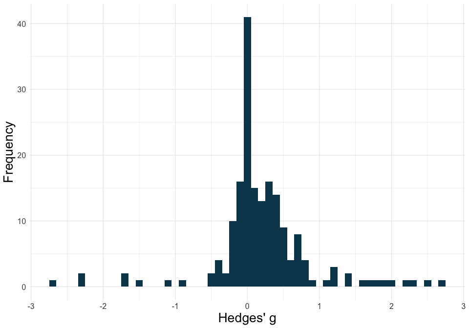
#> 7 NA 13 Cohen's d 0.00 8 0.28 12 0.9361702The esd_plot() function can visualise ESDs based on effect size
estimates obtained from meta-analyses.
library(ESDist)plot1 <- esd_plot(df = ot_dat,
es = yi,
es_type = "Hedges' g")
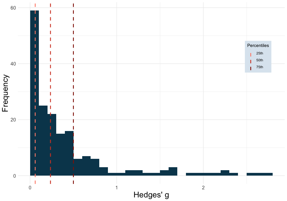
plot1It is also possible to plot effect size benchmarks based on the 25th,
50th, and 75th percentiles by adding method = "quads" (or based on the
16.65th, 50th, and 83.35th percentiles by adding method = "thirds").
plot2 <- esd_plot(df = ot_dat,
                  es = yi,
                  es_type = "Hedges' g",
                  method = "quads")

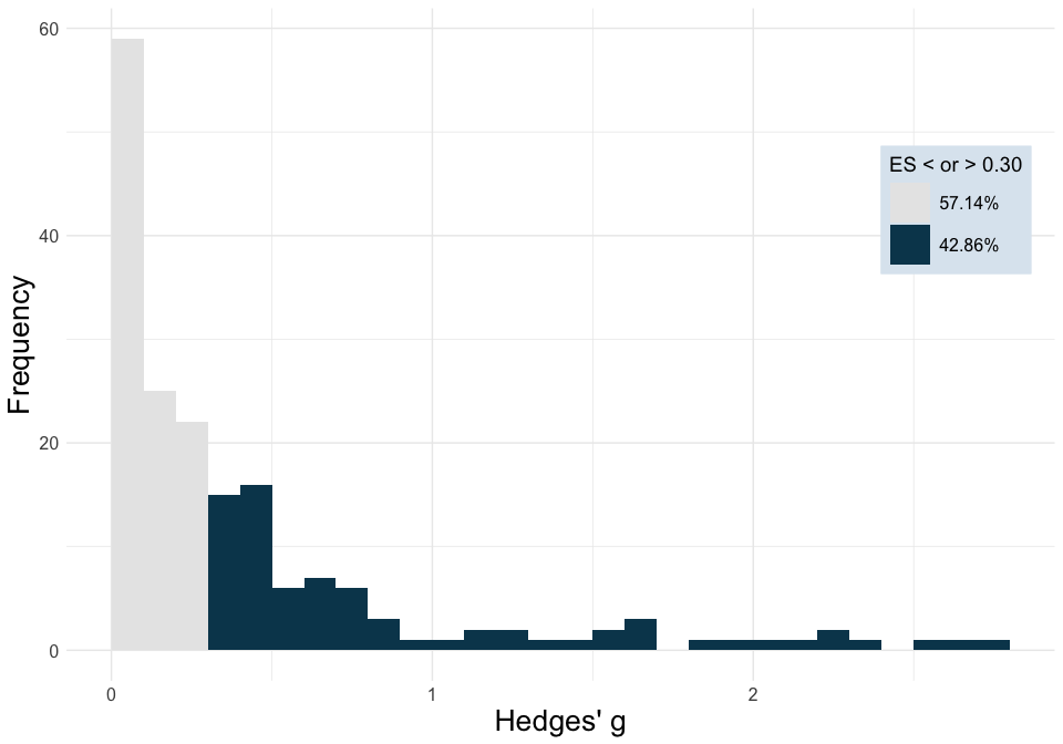
plot2Finally, we can specify the range of effect sizes that is equal to or
larger than a specified sesoi.
plot3 <- esd_plot(df = ot_dat,
                  es = yi,
                  es_type = "Hedges' g",
                  sesoi = 0.3)

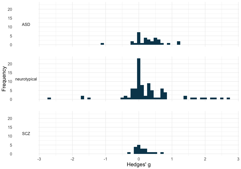
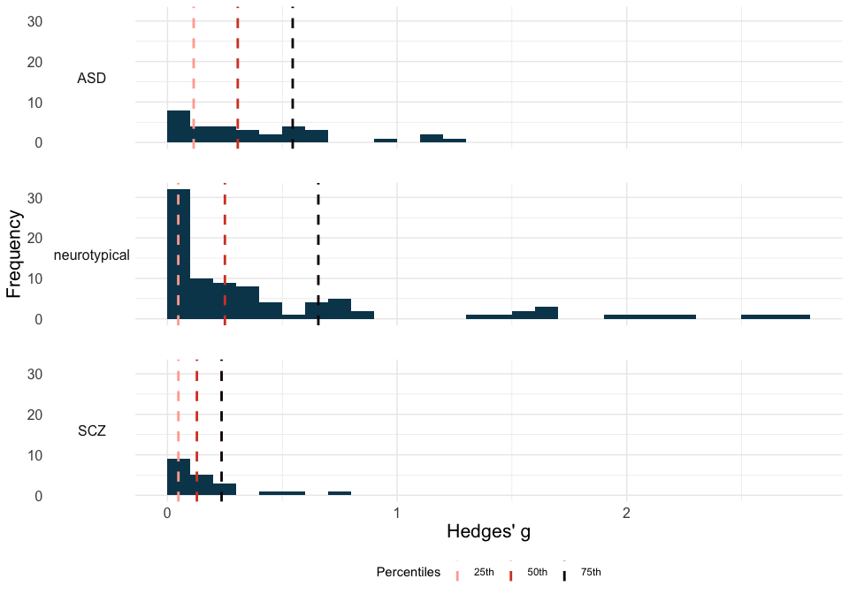
plot3The esd_plot_group() function allows for specifying a grouping_var
to group data and create plots for each group with 20 or more effect
sizes.
plot4 <- esd_plot_group(df = ot_dat,
                        es = yi,
                        es_type = "Hedges' g",
                        grouping_var = group)

plot4Like the esd_plot() function, the esd_plot_group() function lets you
plot effect size benchmarks based on a specific set of percentiles, by
adding method = "quads" or method = "thirds".
plot5 <- esd_plot_group(df = ot_dat,
                        es = yi,
                        es_type = "Hedges' g",
                        grouping_var = group,
                        method = "quads")

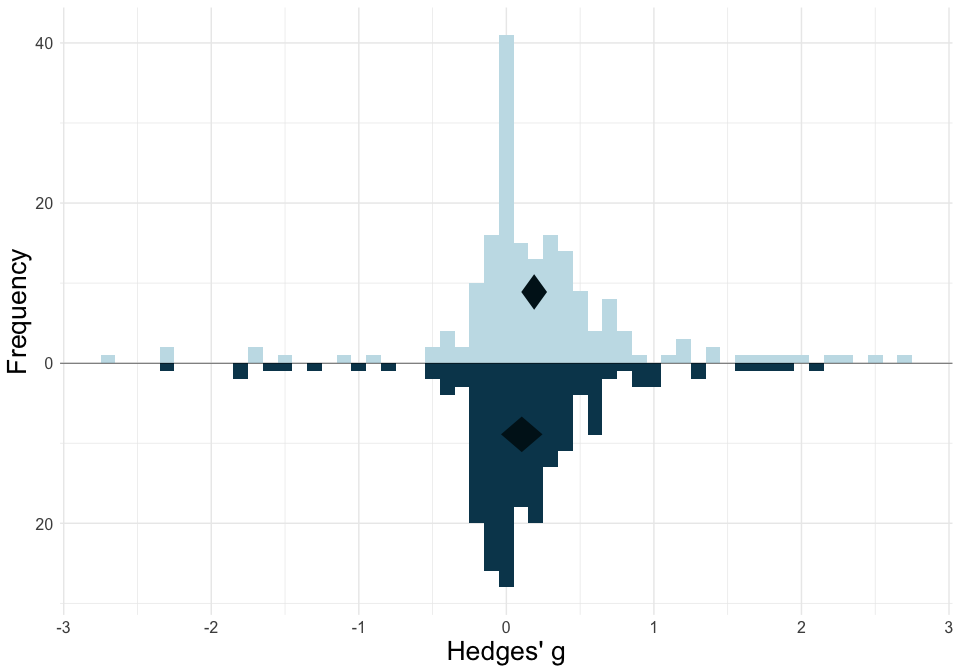
plot5Using limit meta analysis (Schwarzer et al., 2023), we can adjust every
individual effect size for publication bias and plot the adjusted
distribution against the raw distribution. To do this, the
esd_plot_pba() function takes an additional se argument.
plot6a <- esd_plot_pba(df = ot_dat,
                       es = yi,
                       se = sei,
                       es_type = "Hedges' g")

plot6a
For more control over the parameters of the limit meta-analysis, it is
possible to install the meta and metasens packages and creating a
limitmeta object. The esd_plot_pba() function can then take a
lim_obj argument instead of df, es, and se arguments.
library(meta)
library(metasens)

m1 <- metagen(TE = ot_dat$yi, seTE = ot_dat$sei)
l1 <- limitmeta(m1)

plot6b <- esd_plot_pba(lim_obj = l1,
                       es_type = "Hedges' g")

plot6b
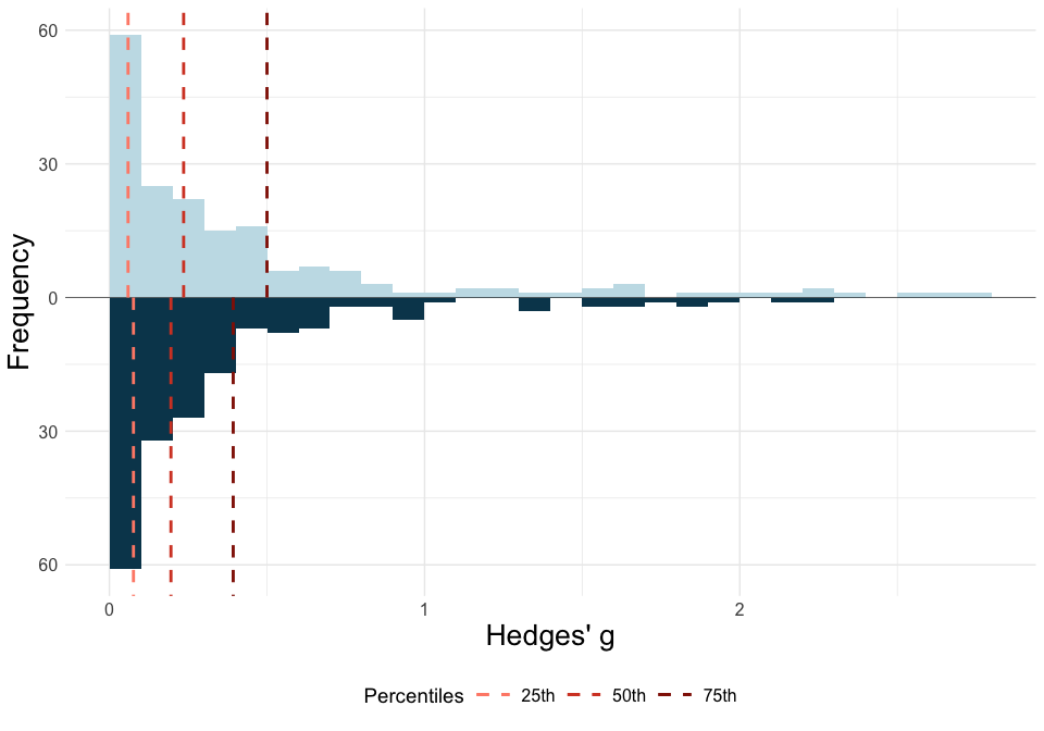
Alternatively, we can plot the effect size benchmarks for both distributions.
plot7 <- esd_plot_pba(df = ot_dat,
                      es = yi,
                      se = sei,
                      es_type = "Hedges' g",
                      method = "quads")

plot7
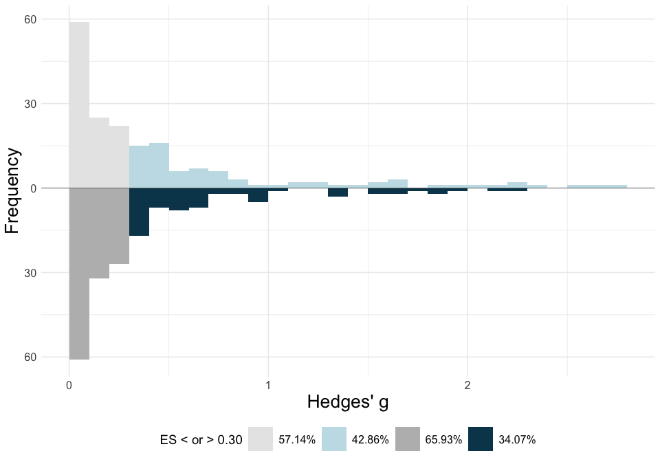
Or the range of effect sizes larger than or equal to a SESOI
plot8 <- esd_plot_pba(df = ot_dat,
                      es = yi,
                      se = sei,
                      es_type = "Hedges' g",
                      sesoi = 0.3)
plot8By using the esd_table() function, you can calculate the effect size
benchmarks for your dataset by specifying the dataset (df), and the
column containing all effect sizes (es). This will give you the effect
size benchmarks based on the 25th, 50th, and 75th percentiles.
library(ESDist)
library(dplyr)
table1 <- esd_table(df = ot_dat,
es = yi)
table1
#> 25% 50% 75% Number of effects
#> Raw effect size 0.06 0.24 0.5 182By specifying grouping_var, the user can calculate the effect size
benchmarks per group, for every group with at least three effect sizes.
(The number of required effect sizes per group can be overwritten by
specifying min_group_size.)
table3 <- esd_table(df = ot_dat,
                    es = yi,
                    grouping_var = group)

table3
#>          Group  25%  50%  75% Number of effects
#> 1           AN 0.02 0.05 0.06                 6
#> 2          ASD 0.11 0.31 0.55                32
#> 3          BPD 0.16 1.22 2.29                 5
#> 4         PTSD 0.20 0.32 0.38                 6
#> 5          SCZ 0.05 0.13 0.24                20
#> 6      anxiety 0.19 0.31 0.41                 4
#> 7   depression 0.21 0.45 0.91                 6
#> 8 neurotypical 0.05 0.25 0.66                89
#> 9 All 0.06 0.24 0.50 182The esd_table_pba() function, similar to the esd_plot_pba()
function, allows users to calculate effect size benchmarks that are
adjusted for publication bias.
table4 <- esd_table_pba(df = ot_dat,
                        es = yi,
                        se = sei)

table4
#>                       25%  50%  75% Number of effects
#> Raw effect size      0.06 0.24 0.50               182
#> Adjusted effect size 0.08 0.20 0.39               182
In case the user wants effect size benchmarks per group, the user should
define the grouping_var argument:
table5 <- esd_table_pba(df = ot_dat,
                        es = yi,
                        se = sei,
                        grouping_var = group)

table5
#>                        25%  50%  75% Number of effects
#> AN                    0.02 0.05 0.06                 6
#> AN adjusted           0.04 0.07 0.09                 6
#> ASD                   0.11 0.31 0.55                32
#> ASD adjusted          0.10 0.23 0.39                32
#> BPD                   0.16 1.22 2.29                 5
#> BPD adjusted          0.19 0.92 1.82                 5
#> PTSD                  0.20 0.32 0.38                 6
#> PTSD adjusted         0.12 0.22 0.29                 6
#> SCZ                   0.05 0.13 0.24                20
#> SCZ adjusted          0.08 0.15 0.18                20
#> anxiety               0.19 0.31 0.41                 4
#> anxiety adjusted      0.06 0.21 0.36                 4
#> depression            0.21 0.45 0.91                 6
#> depression adjusted   0.14 0.37 0.72                 6
#> neurotypical          0.05 0.25 0.66                89
#> neurotypical adjusted 0.06 0.20 0.55                89
#> All                   0.06 0.24 0.50               182
#> All adjusted 0.08 0.20 0.39 182The values presented in the table default to two decimal places. This
can be overwritten by setting ndec to the desired number of decimal
places. Tables can be saved by setting csv_write to TRUE.
Optionally, by setting file_name to a string specifying the
sub-directory and file name (e.g., sub-folder/table.csv), the table
can be saved to a specific location with a specific name.
Using esd_perc(), you can calculate to which percentile of the ESD a
given value corresponds. Note that absolute effect size values should be
used.
library(ESDist)
library(dplyr)
library(ggplot2)esd_perc(df = ot_dat,
es = yi,
value = 0.3)
#> [1] 57.14286