bernsblack / hawkes

Python class for generation and parameter estimation of multivariate Hawkes processes

Python class for Multivariate Hawkes Processes

This repo provides a class MHP for doing basic experimentation with a Hawkes process. It works for both uni- and multivariate processes, and implements both synthetic sequence generation and parameter estimation of a known sequence. I use a MAP EM algorithm for parameter estimation that is described in this unpublished report for the univariate case, and my masters thesis for the multivariate case.

There is a blog post here describing more details, such as theoretical preliminaries and some suggested usage and further reading.

Contents

The MHP.py file contains a single class, MHP. The core methods are:

1. generate_seq: generates synthetic sequences given parameter values specified in the constructor. Uses Ogata thinning with two speedups/modifications: it saves the rates at the moment of the last event, and it does the "attribution/rejection" test as a weighted random sample (using NumPy's random.sample) instead of, e.g., a for-loop.

2. EM: uses a Bayesian EM algorithm to learn parameters, given a sequence and estimates of alpha, mu, and omega. It treats omega as a hyperparameter and does not optimize over this parameter. For more details see the report, my thesis, or this blog post.

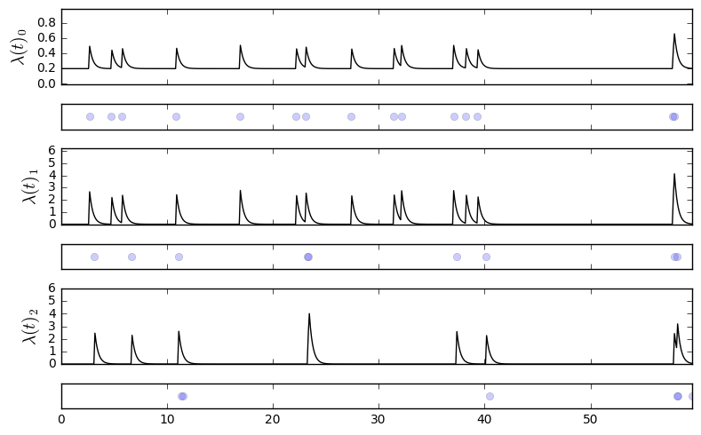
There are also two visualization methods, plot_events (which plots only the time series of events), and plot_rates (which plots the time series with the corresponding conditional intensities, currently only implemented for dim=3).

Usage

You can test basic functionality using default parameters as follows:

from MHP import MHP
P = MHP()
P.generate_seq(60)

which will initialize a univariate process with parameters mu=[0.1], alpha=[[0.5]], and omega=1.0. This sequence is stored as P.data, a numpy.ndarray with 2 columns: the first column with the timestamps, the second with the stream assignment (in this case there is only one stream).

You can then plot the events with

P.plot_events()

For a more interesting test, try engineering your own parameters. Here is an example with dim=3:

m = np.array([0.2, 0.0, 0.0])
a = np.array([[0.1, 0.0, 0.0], 
              [0.9, 0.0, 0.0],
              [0.0, 0.9, 0.0]])
w = 3.1

P = MHP(mu=m, alpha=a, omega=w)
P.generate_seq(60)
P.plot_events()

We can also look at the conditional intensities along with the time series of events:

We can learn the parameters of an already generated sequence by simply calling EM with some guesses at alpha and mu (and a hyperparameter omega),

mhat = np.random.uniform(0,1, size=3)
ahat = np.random.uniform(0,1, size=(3,3))
w = 3.

P.EM(ahat, mhat, w)

which will give output something like:

After ITER 0 (old: -10000.000 new: -0.129)
 terms 5.1766, 17.4638, 8.5362
After ITER 10 (old: -0.129 new: -1.349)
 terms -20.8908, 11.8172, 14.1828
Reached stopping criterion. (Old: -1.349 New: -1.350)

(array([[ 0.0223,  0.1475,  0.    ],
        [ 0.5954,  0.    ,  0.    ],
        [ 0.    ,  0.625 ,  0.    ]]), 
 array([ 0.2038,  0.0046,  0.    ]))

This is already a reasonable approximation to the actual ground truth values from above, without including regularization, cross-validation, a larger sample, etc.

Summary

This is a bare bones collection of code that is hopefully helpful to someone dipping his/her toes in the waters of multivariate point processes. For more robust packages, or a more indepth look at behind-the-scenes, check out this blog post which covers some basic theoretical concepts and also links to some other more expansive code repos out there.