regimeshifts

regimeshifts is a Python library that contains useful functions to detect early warning signals for an approaching regime shift on a time-series.

The indicators implemented in this library are lag-1 autocorrelation and variance. The rationale behind these indicators is based on a phenomenon known as Critical Slowing Down: as a system approaches gradually a tipping point, its recovery rate from perturbations decreases leading to an increase in similarity over time. Those changes can be detected by measuring changes in lag-1 autocorrelation and variance. Usually a tipping point is preceded by an increase in both metrics, if approached gradually (see Scheffer et al. (2009)).

Since these metrics do not constitute a forecast tool to predict the distance to the tipping point, they are regarded as indicators of resilience and/or stability of a system (see Dakos et al. (2015)).

Note: This library is still under development, although the implemented methods are fairly tested.

Modules

regimeshifts contains two modules:

ews: Contains useful methods to compute the resilience indicators, their robustness and significance.
regime_shifts: Contains a method to detect regime shifts in a time-series.

This repository can be copied into the working directory using the command:

https://github.com/BeatrizArellano/regimeshifts.git

Both modules can be imported as follows (assuming the folder regimeshifts is at the same level of the script in which they are imported):

from regimeshifts import regime_shifts as rs
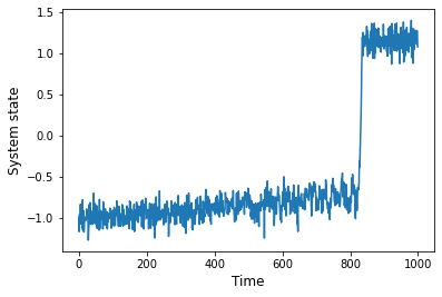
from regimeshifts import ews

Creating a time-series with a tipping point

sample_rs is a useful function in the module regime_shifts to create a time-series with a bifurcation and stochastic variability (normally distributed noise with specified standard deviation).

ts = rs.sample_rs(std=0.1)

import matplotlib.pyplot as plt
fig, ax = plt.subplots()
ts.plot(ax=ax)
ax.set_xlabel('Time',fontsize=12)
ax.set_ylabel('System state',fontsize=12);

Detecting regime shifts

The class Regime_shift contains a useful method proposed by Boulton and Lenton (2019) to detect regime shifts in a time-series. This method looks for gradient changes that occur overa small time interval.

First, we create an instance of the class Regime_shifts passing a pandas time-series as a parameter.

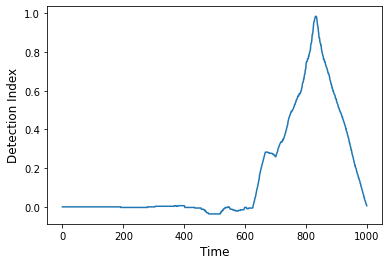
ts = rs.Regime_shift(ts)

The method as_detect computes the detection indices returning a time-series containing values in the interval [-1,1] along the time-series. The greatest (smallest) values may indicate the occurrence of a regime shift. In this example, the largest value is detected exactly when the tipping point is reached in the original series.

detection_index = ts.as_detect()

fig, ax = plt.subplots()
detection_index.plot(ax=ax)
ax.set_xlabel('Time',fontsize=12)
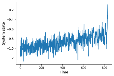
ax.set_ylabel('Detection Index',fontsize=12);

The before_rs method can be used to extract the data before the regime-shift:

bef_rs = ts.before_rs()

fig, ax = plt.subplots()
bef_rs.plot(ax=ax)
ax.set_xlabel('Time',fontsize=12)
ax.set_ylabel('System state',fontsize=12);

Early warning signals (resilience indicators)

From the proposed indicators for Critical Slowing Down in the literature, we included methods to measure temporal lag-1 autocorrelation and variance. The time-series are usually detrended prior to estimating the indicators (see Lenton et al. (2012)).

The class Ews (stands for Early Warning Signals) contains the methods to detrend the time-series, estimate the resilience indicators, measure the strength of change in their trend over time, their robustness and significance.

First, we create an instance of the class Ews passing a Pandas time-series or dataframe as parameter.

Here we use the portion of the sample series before the regime shift.

series = ews.Ews(bef_rs)
series = series.rename(columns={0:'Sample series'}) ## The Ews class returns an extended Dataframe object, if we provided a series, it sets 0 for the column name.

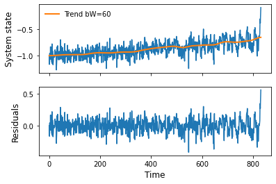
The method gaussian_det can be used to remove the trend using a moving average weighed by a Gaussian function (or a Gaussian kernel smoother), which receives the bandwidth (bW) of the Gaussian smoother kernel as a parameter (see Lenton et al. (2012)).

This method returns a class containing the attributes: trend and res (residuals).

trend = series.gaussian_det(bW=60).trend
residuals = series.gaussian_det(bW=60).res

fig, axs = plt.subplots(2,1,sharex=True)
bef_rs.plot(ax=axs[0],label='')
trend['Sample series'].plot(ax=axs[0],label='Trend bW=60',linewidth=2)
residuals['Sample series'].plot(ax=axs[1])
axs[1].set_xlabel('Time',fontsize=12)
axs[0].set_ylabel('System state',fontsize=12);
axs[1].set_ylabel('Residuals',fontsize=12);
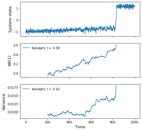
axs[0].legend(frameon=False);

Estimating autocorrelation and variance

From the proposed indicators for Critical Slowing Down in the literature, we included methods to measure lag-1 autocorrelation and variance on time-series. They are computed over a sliding window with a size determined by the user (parameter wL). The sliding window can be set as a number of data points or as a proportion of the time series (e.g. wL=0.5). These methods can be applied over the detrended data or they can be applied directly to the raw data, in which the detrending step can be applied by setting detrend=True and providing the bandwidth size (bW).

The methods to compute lag-1 autocorrelation are: ar1(), which fits an autoregressive model of order 1, and pearsonc(). The method var() computes variance.

wL = 200 ## Window length specified in number of points in the series
bW = 60
ar1 = series.ar1(detrend=True,bW=bW,wL=wL) ### Computing lag-1 autocorrelation using the ar1() method
var = series.var(detrend=True,bW=bW,wL=wL) ## Computing variance

Measuring the trend in the indicators with the non-parametric Kendall's $\tau$ correlation coefficient

The Kendall $\tau$ coefficient cross-correlates time and the indicator series to assess the strength of change over time. The resulting coefficient ranges between -1 and 1: where values close to 1 indicate an increasing trend, and -1 a decreasing trend (see Lenton et al. (2012)).

The Kendall coefficient is an attribute of the resulting indicator series and it is computed in this way:

series.ar1(detrend=True,bW=bW,wL=wL).kendall.

print(f'AR(1) tau = {ar1.kendall:0.3f}')
print(f'Var tau = {var.kendall:0.3f}')

AR(1) tau = 0.899
Var tau = 0.628

fig, axs = plt.subplots(3,1,sharex=True,figsize=(7,7))
ts.plot(ax=axs[0],legend=False)
ar1['Sample series'].plot(ax=axs[1],label=rf"Kendall's $\tau =$ {ar1.kendall:.2f}")
var['Sample series'].plot(ax=axs[2],label=rf"Kendall's $\tau =$ {var.kendall:.2f}")
axs[0].set_ylabel('System state',fontsize=13)
axs[1].set_ylabel('AR(1)',fontsize=13)
axs[2].set_ylabel('Variance',fontsize=13)
axs[1].legend(frameon=False)
axs[2].legend(frameon=False)
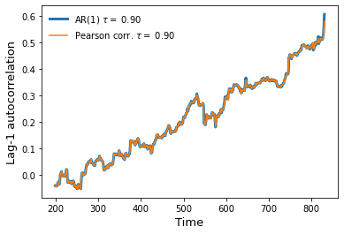
axs[2].set_xlabel('Time',fontsize=13);

AR(1) vs Pearson Correlation Coefficient

The method ar1() fits a first-order autoregressive model (AR(1)) using an ordinary least-squares method. This method uses the statsmodels AutoReg function, which is relatively computationally expensive compared with computing the Pearson correlation coefficient. The method pearsonc uses the Pandas autocorr function to estimate the correlation beween the time-series comprised by the window and the same time-series shifted by one time-unit.

As we can see in this section, both methods yield the same results.

pearson = series.pearsonc(detrend=True,bW=bW,wL=wL) ### Computing lag-1 autocorrelation using the pearsonc() method

fig,axs = plt.subplots()
ar1['Sample series'].plot(ax=axs,linewidth=3,label=rf"AR(1) $\tau =$ {ar1.kendall:.2f}")
pearson['Sample series'].plot(ax=axs,label=rf"Pearson corr. $\tau =$ {pearson.kendall:.2f}")
axs.legend(frameon=False)
axs.set_ylabel('Lag-1 autocorrelation',fontsize=13)
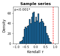
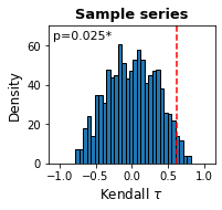
axs.set_xlabel('Time',fontsize=13);

Assessing significance

A proposed method to measure whether a trend is significant consists in comparing the measured trend with the expected trends from a null model. The null model consists of a large-enough number of surrogate series, each series having the same spectral properties as the original series (see Dakos et al. (2012)). This can be achieved by using a bootstrapping method: sampling with replacement from the residuals of the original time-series (see Boulton et al. (2014)). The Kendall $\tau$ coefficient is measured for each surrogate series and the $p$-value is then defined as the proportion of series that exhibit a $\tau$-value greater (smaller) than or equal to that observed in the original series.

The function significance follows this method to return an object with the following attributes:

indicator: The resilience indicator
surrog_kendalls: a Pandas dataframe containing the Kendall values measured on each surrogate series.
kendall_coeff: The Kendall coefficient for the indicator's trend computed on the original series
pvalue: The p-value
test_type: Positive or negative, defined to assess whether the trend is significantly positive or negative.
plot(): Method to plot the output from the test.

sig_pearson = series.significance(indicator='pearsonc',n=1000,detrend=True,wL=wL,bW=bW,test='positive')

sig_variance = series.significance(indicator='var',n=1000,detrend=True,wL=wL,bW=bW,test='positive')

sig_variance.pvalue

Sample series    0.025
dtype: float64

print(f'Lag-1 autocorrelation p-value: {sig_pearson.pvalue["Sample series"]}')
print(f'Variance p-value: {sig_variance.pvalue["Sample series"]}')

Lag-1 autocorrelation p-value: 0.0
Variance p-value: 0.025

Visualising the significance test

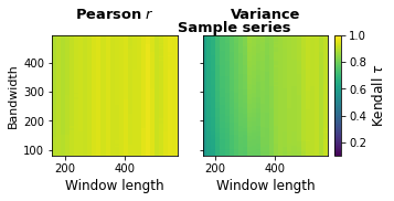
The plot() method plots the distribution of Kendall $\tau$ values obtained from the surrogate series and a red vertical line that indicates the Kendall coefficient measured on the original series.

sig_pearson.plot()

sig_variance.plot()

Robustness analysis

The method robustness() measures the trends for the specified indicators over a range of combinations of window lengths and detrending bandwidths.

This method receives as parameters the indicators to assess, the minimum and maximum window length (min_wL and max_wL) as well as its resolution (res_wL). Likewise for the detrending bandwidth (min_bW,max_bW,res_bW).

This method returns a dictionary in which the keys correspond to the dataframe column names. Each key is associated to another dictionary containing Pandas dataframes with the Kendall values across all the combination of parameters (The columns corresponding to each window size and the indices to the different bandwidths).

rob = series.robustness(indicators=['pearsonc','var'])

rob['Sample series']['pearsonc']

.dataframe tbody tr th {
    vertical-align: top;
}

.dataframe thead th {
    text-align: right;
}

</style>

	166	181	196	211	226	241	256	271	286	301	...	436	451	466	481	496	511	526	541	556	571
Bandwidth
83	0.897880	0.906709	0.898202	0.908233	0.921512	0.930012	0.929239	0.924153	0.931068	0.945351	...	0.942360	0.941484	0.959159	0.971282	0.955082	0.929167	0.939698	0.955682	0.963109	0.961273
88	0.898539	0.906728	0.898450	0.908597	0.921054	0.929634	0.929300	0.924281	0.931095	0.945379	...	0.942488	0.941484	0.959219	0.971282	0.955402	0.929517	0.939698	0.955872	0.963109	0.961096
93	0.898864	0.907068	0.898351	0.908805	0.920825	0.929232	0.929203	0.924191	0.931001	0.945535	...	0.942463	0.941567	0.959368	0.971412	0.955544	0.929361	0.939912	0.955966	0.963215	0.960743
98	0.898855	0.907078	0.898192	0.908826	0.920705	0.928934	0.929130	0.924141	0.930961	0.945649	...	0.942411	0.941484	0.959398	0.971445	0.955579	0.929322	0.939569	0.955919	0.963162	0.960566
103	0.898711	0.907068	0.898321	0.908981	0.920541	0.928613	0.929130	0.924141	0.930974	0.945663	...	0.942360	0.941428	0.959219	0.971282	0.955757	0.929206	0.939312	0.955872	0.963320	0.960389
...	...	...	...	...	...	...	...	...	...	...	...	...	...	...	...	...	...	...	...	...	...
473	0.891829	0.906426	0.896479	0.903039	0.916974	0.927454	0.933104	0.924497	0.930141	0.944128	...	0.938524	0.941539	0.956853	0.968352	0.949609	0.927375	0.936783	0.952648	0.961476	0.958680
478	0.891811	0.906426	0.896519	0.903101	0.916963	0.927512	0.933043	0.924382	0.930114	0.944100	...	0.938345	0.941539	0.956913	0.968254	0.949183	0.927220	0.936869	0.952601	0.961370	0.958680
483	0.891621	0.906530	0.896509	0.903049	0.916963	0.927546	0.933128	0.924230	0.930127	0.944086	...	0.938371	0.941622	0.956973	0.968059	0.948934	0.927336	0.936783	0.952601	0.961370	0.958680
488	0.891504	0.906567	0.896469	0.903028	0.916995	0.927546	0.933128	0.924166	0.930262	0.944071	...	0.938294	0.941484	0.957003	0.967896	0.948756	0.927142	0.936783	0.952364	0.961159	0.958562
493	0.891323	0.906577	0.896390	0.902956	0.916984	0.927569	0.933056	0.924026	0.930235	0.944000	...	0.938115	0.941345	0.957033	0.967993	0.948579	0.927064	0.936869	0.952506	0.961265	0.958562

83 rows × 28 columns

Robustness figures

The robustness results can be represented as colourmaps by using the plot() method. In this method, the parameters vmin,vmax,cmap and other arguments for the Matplotlib pcolormesh function can be specified.

rob.plot(vmin=0.1,cmap='viridis')

References

Boulton, C. A., & Lenton, T. M. (2019). A new method for detecting abrupt shifts in time series. F1000Research, 8, 746. https://doi.org/10.12688/f1000research.19310.1
Boulton, C. A., Allison, L. C., & Lenton, T. M. (2014). Early warning signals of Atlantic Meridional Overturning Circulation collapse in a fully coupled climate model. Nature Communications, 5(1), 1–9. https://doi.org/10.1038/ncomms6752
Dakos, V., Carpenter, S. R., van Nes, E. H., & Scheffer, M. (2015). Resilience indicators: Prospects and limitations for early warnings of regime shifts. Philosophical Transactions of the Royal Society B: Biological Sciences, 370(1659), 20130263. https://doi.org/10.1098/rstb.2013.0263
Dakos, V., Carpenter, S. R., Brock, W. A., Ellison, A. M., Guttal, V., Ives, A. R., Kéfi, S., Livina, V., Seekell, D. A., van Nes, E. H., & Scheffer, M. (2012). Methods for Detecting Early Warnings of Critical Transitions in Time Series Illustrated Using Simulated Ecological Data. PLoS ONE, 7(7), e41010. https://doi.org/10.1371/journal.pone.0041010
Lenton, T. M., Livina, V. N., Dakos, V., van Nes, E. H., & Scheffer, M. (2012). Early warning of climate tipping points from critical slowing down: Comparing methods to improve robustness. Philosophical Transactions of the Royal Society A: Mathematical, Physical and Engineering Sciences, 370(1962), 1185–1204. https://doi.org/10.1098/rsta.2011.0304
Scheffer, M., Bascompte, J., Brock, W. A., Brovkin, V., Carpenter, S. R., Dakos, V., Held, H., van Nes, E. H., Rietkerk, M., & Sugihara, G. (2009). Early-warning signals for critical transitions. Nature, 461(7260), 53–59. https://doi.org/10.1038/nature08227

bassemfg / regimeshifts