Steven Moran and Adriano Lameira
(06 February, 2023)
This RMarkdown report contains supplementary materials for the manuscript “Life of p: A consonant older than speech”. It uses the R programming language (R Core Team 2021) and the following R libraries (Wickham et al. 2019; Xie 2021; Revell 2012; J. Zhang 2017; Yu 2020; Wickham 2011):
library(tidyverse)
library(knitr)
library(phytools)
library(phylotools)
library(ggtree)
library(testthat)
In what follows, we undertake several analyses including:
- Investigating the cross-linguistic frequency of labial segments including /p/ and /b/ in a large sample of the world’s languages
- Examining how common the contrastive feature labial is in the documented phonological inventories of the world
- Identifying the presence of labial segments in ancient and reconstructed languages
- Looking at labials in language families from a diachronic perspective, i.e., investigating whether they are prominent or not within large language families for which we have robust computational phylogenetics data
For cross-linguistic analyses of segment frequencies, we combine the PHOIBLE sample of phonological inventories (Moran and McCloy 2019) and append to them the linguistic and non-linguistic metadata data associated with the Glottolog, a catalog of the world’s languages (Hammarström et al. 2020).
phoible <- read_csv(url("https://github.com/phoible/dev/blob/646f5e4f64bfefb7868bf4a3b65bcd1da243976a/data/phoible.csv?raw=true"),
  col_types = c(InventoryID = "i", Marginal = "l", .default = "c")
)

glottolog <- read_csv(url("https://cdstar.shh.mpg.de/bitstreams/EAEA0-E62D-ED67-FD05-0/languages_and_dialects_geo.csv"))

phoible <- left_join(phoible, glottolog, by = c("Glottocode" = "glottocode"))
The data look like this.
phoible %>%
  select(InventoryID, LanguageName, Phoneme) %>%
  head() %>%
kable()| InventoryID | LanguageName | Phoneme |
|---|---|---|
| 1 | Korean | h |
| 1 | Korean | j |
| 1 | Korean | k |
| 1 | Korean | kʰ |
| 1 | Korean | kˀ |
| 1 | Korean | l |
How many inventories (data points) are there in PHOIBLE?
nrow(phoible %>% select(InventoryID) %>% distinct())## [1] 3020
How many languages (defined as distinct ISO 639-3 language identifiers) are there?
nrow(phoible %>% select(ISO6393) %>% distinct())## [1] 2093
How many segment types are there?
nrow(phoible %>% select(Phoneme) %>% distinct())## [1] 3169
Get all rows with phonemes that are voiceless bilabial plosive, i.e., “p” like.
df <- phoible %>% filter(grepl("p", Phoneme))What are they?
ps <- df %>%
  select(Phoneme) %>%
  distinct()
ps <- df %>%
  select(Phoneme) %>%
  group_by(Phoneme) %>%
  summarize(count = n()) %>%
  arrange(desc(count))
head(ps) %>% kable()| Phoneme | count |
|---|---|
| p | 2594 |
| pʰ | 592 |
| kp | 373 |
| pʼ | 178 |
| p͉ | 79 |
| p͈ | 72 |
# write_csv(ps, 'ps.csv')Some of the “p-like” segments include labiovelars like /kp/. Let’s drop those.
ps <- ps %>% filter(!(grepl("kp|pf|mp", Phoneme)))Since PHOIBLE may have multiple analyses for the same language variety (see explanation regarding so-called “doculects” in the PHOIBLE FAQ), we combine the phonological inventories from multiple sources into single entries so that we can examine which languages have been reported to have certain segments or not.
phoible_by_iso <- phoible %>%
  select(ISO6393, Phoneme) %>%
  group_by(ISO6393) %>%
  distinct()
Since the ISO 6393 code mis is for languages that are missing a
language name identifier, we drop those.
phoible_by_iso <- phoible_by_iso %>% filter(ISO6393 != "mis")How many distinct languages are left once they have been aggregated by ISO 639-3 code?
num_languages <- nrow(phoible_by_iso %>% distinct(ISO6393))
num_languages
## [1] 2092
Now we select from these languages which have a p-like segment.
phoible_by_iso_with_p <- phoible_by_iso %>% filter(Phoneme %in% ps$Phoneme)
phoible_by_iso_with_p %>%
  head() %>%
kable()| ISO6393 | Phoneme |
|---|---|
| kor | p |
| kor | pʰ |
| kor | pˀ |
| lbe | pʰ |
| lbe | pʼ |
| lbe | p͈ |
We summarize their counts.
phoible_by_iso_with_p %>%
  group_by(ISO6393) %>%
  summarize(n = n()) %>%
  arrange(desc(n))
## # A tibble: 1,949 × 2
## ISO6393 n
## <chr> <int>
## 1 lez 6
## 2 sjd 6
## 3 bcq 5
## 4 gle 5
## 5 lbe 5
## 6 yey 5
## 7 acn 4
## 8 ahk 4
## 9 alw 4
## 10 amh 4
## # … with 1,939 more rows
And ask what percentage of languages in PHOIBLE have p-like sounds.
nrow(phoible_by_iso_with_p %>% select(ISO6393) %>% distinct()) / num_languages## [1] 0.9316444
Which are the languages that contain no “p-like” segments?
phoible_by_iso_no_p <- phoible_by_iso %>%
  filter(!(ISO6393 %in% phoible_by_iso_with_p$ISO6393)) %>%
  select(ISO6393) %>%
  distinct() %>%
  arrange(ISO6393)

phoible_by_iso_no_p %>%
  head() %>%
kable()| ISO6393 |
|---|
| aar |
| aey |
| aft |
| aha |
| aht |
| aiw |
There are quite a few languages without “p-like” segments.
nrow(phoible_by_iso_no_p)## [1] 143
Or about 7% of languages in the sample (see above).
nrow(phoible_by_iso_no_p) / num_languages## [1] 0.06835564
One random example is Afar, which does not contain a voiceless bilabial plosive, but it does contain its voiced counterpart “b”. Another is Somali with the same segment configuration within the bilabial plosives. Both languages are also in Africa.
Let’s look geographically at which languages lack voiceless bilabial plosives.
no_p_by_geography <- phoible %>%
  filter(ISO6393 %in% phoible_by_iso_no_p$ISO6393) %>%
  select(ISO6393, latitude, longitude, macroarea) %>%
  distinct() %>%
  arrange(ISO6393)
How do these language points look on a map? There are no data points in Eurasia nor Australia, but many in Oceania, Africa, and South America.
ggplot(data = no_p_by_geography, aes(x = longitude, y = latitude)) +
  borders("world", colour = "gray50", fill = "gray50") +
  geom_point()
Africa is notable for lacking voiceless bilabial plosives (Houis 1974; Maddieson 1984; Clements and Rialland 2008) and is interesting because within a relatively broad sample of phonological segment borrowings /p/ is the most frequently borrowed speech sound (Grossman et al. 2020). In other words, /p/ seems to have been lost in certain linguistic areas, probably due to regular processes of sound change, but then is easily re-introduced into languages via borrowing, e.g., Tem (Central Gur, Togo), Tigrinya (Semitic, Ethiopia), or !Xóõ (Tuu, Botswana and Namibia) (Clements and Rialland 2008). (Similar observations about cross-linguistically frequently segments missing in certain world areas, which were perhaps lost at some point in the past and this loss then inherited by daughter languages and dialects, is reported by Moran, Lester, and Grossman (2021)).
So of the languages that lack /p/, how many also lack /b/?
tmp <- phoible_by_iso %>% filter(ISO6393 %in% phoible_by_iso_no_p$ISO6393)
tmp <- tmp %>% filter(grepl("b", Phoneme))
tmp <- tmp %>% filter(!grepl("ɡb", Phoneme)) # Let's drop labial velars
tmp <- tmp %>%
  select(ISO6393) %>%
  distinct() %>%
  arrange(ISO6393)
tmp <- phoible_by_iso_no_p %>% filter(!(ISO6393 %in% tmp$ISO6393))
tmp %>% kable()| ISO6393 |
|---|
| bvi |
| chr |
| eya |
| kam |
| kuj |
| mch |
| ndh |
| one |
| opy |
| tcb |
| trr |
| unk |
| waw |
| wic |
| wya |
Where are they spoken?
no_bilabials <- phoible %>%
  filter(ISO6393 %in% tmp$ISO6393) %>%
  select(ISO6393, latitude, longitude, macroarea) %>%
  distinct() %>%
  arrange(macroarea)
no_bilabials %>% kable()| ISO6393 | latitude | longitude | macroarea |
|---|---|---|---|
| kuj | -1.50636 | 34.50490 | Africa |
| bvi | 7.41311 | 27.69560 | Africa |
| kam | -1.60827 | 37.95320 | Africa |
| ndh | -9.88948 | 33.61180 | Africa |
| wic | 35.06650 | -98.18310 | North America |
| one | 43.43874 | -75.70811 | North America |
| chr | 35.46640 | -83.16300 | North America |
| eya | 60.42320 | -144.76200 | North America |
| wya | NA | NA | North America |
| tcb | 63.40460 | -143.33800 | North America |
| unk | -12.43020 | -58.98020 | South America |
| mch | 4.70705 | -64.38770 | South America |
| waw | 1.50881 | -59.14170 | South America |
| trr | -3.22497 | -75.56030 | South America |
| opy | -22.27800 | -53.72270 | South America |
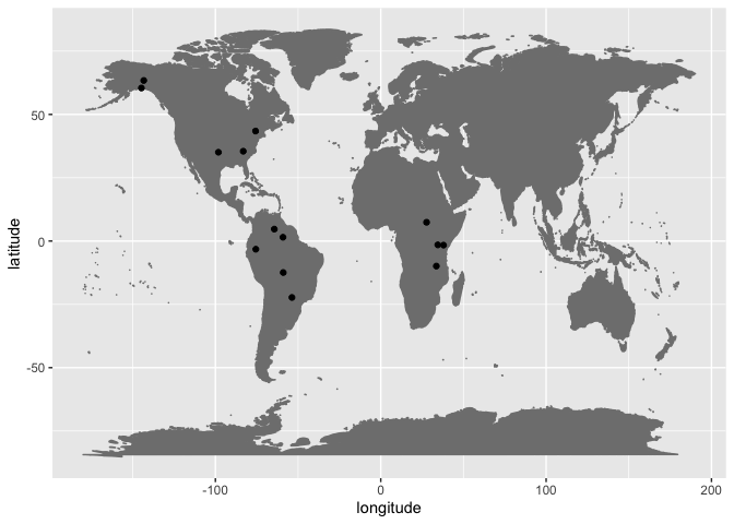
They are mainly found in the Americas.
ggplot(data = no_bilabials, aes(x = longitude, y = latitude)) +
  borders("world", colour = "gray50", fill = "gray50") +
  geom_point()
Languages lacking native bilabial plosives /p/ and /b/ are extremely rare in the PHOIBLE sample overall, i.e. 14 observations out of 2092 languages (0.007%). They include North American languages like Cherokee and Eyak that lack labials except the nasal /m/, which is reportedly rare or only occur in loanwords:
And Wichita with a cross-linguistically unusual phonology that lacks pure labials (e.g., /p/, /b/, and /m/), although it has the voiced labial-velar approximant /w/ and the labiovelar /kʷ/.
In East Africa, the languages include Kikamba, Kuria, Chindali, respectively:
- https://phoible.org/inventories/view/1443#tipa
- https://phoible.org/inventories/view/758#tipa
- https://phoible.org/inventories/view/1471#tipa
Kikamba and Kuria both have a phonemic voiced bilabial fricative /β/ and bilabial nasal /m/. Chindali has /m/, but lacks the voiceless and voiced plosive – although it has the rare labiodental approximant /ʋ/.
The languages reported in South America, Enawené-Nawé, Yekwana, Waiwai, Taushiro, Ofayé, all contain /w/, and /m/, /β/, or /kʷ/ to various extents.
- https://phoible.org/inventories/view/1818#tipa
- https://phoible.org/inventories/view/1879#tipa
- https://phoible.org/inventories/view/1886#tipa
- https://phoible.org/inventories/view/1936#tipa
- https://phoible.org/inventories/view/1968#tipa
Thus, even when languages lack pure /p/ and /b/, there tends to me to some extent the phonological feature labial still present in the phonological inventory.
What about languages with no labial sounds at all? First let’s get all the languages with labials.
labials <- phoible %>%
  select(ISO6393, Phoneme) %>%
  filter(grepl("p|b|m|ɸ|β|ʙ", Phoneme)) %>%
  distinct()

phoible_by_iso_no_labials <- phoible_by_iso %>%
  filter(!(ISO6393 %in% labials$ISO6393)) %>%
  select(ISO6393) %>%
  distinct() %>%
  arrange(ISO6393)
There are five languages in the total sample that purportedly have no kind of labial, /w/ notwithstanding.
phoible_by_iso_no_labials %>% kable()| ISO6393 |
|---|
| one |
| opy |
| trr |
| wic |
| wya |
- https://phoible.org/inventories/view/77#tipa
- https://phoible.org/inventories/view/1968#tipa
- https://phoible.org/inventories/view/1936#tipa
- https://phoible.org/inventories/view/74#tipa
- https://phoible.org/inventories/view/611#tipa
- https://phoible.org/inventories/view/885#tipa
Of the five languages (and six doculects) listed above, only Oneida does not list the voiced labial-velar approximant /w/ as contrastive. Oneida is noted as being exceptional because it lacks bilabial consonants and labiodental fricatives. However, Oneida reportedly has /w/ and labialized /kw/ (Michelson 1990; Abbott 2006) and even in the source above in phoible (Lounsbury 1953), it is noted that many speakers use the voiceless bilabial fricative or other bilabial or labiodental articulations instead of the voiced velar approximant.
How common is the phonological feature labial in the phonological inventories of the world’s documented languages? The segment data in PHOIBLE contain information about their phonetic properties. For example the bilabial consonants:
phoible %>%
  select(Phoneme, SegmentClass, consonantal, labial, periodicGlottalSource, delayedRelease, nasal) %>%
  filter(Phoneme %in% c("p", "b", "m", "ɸ", "β", "ʙ")) %>%
  distinct() %>%
kable()| Phoneme | SegmentClass | consonantal | labial | periodicGlottalSource | delayedRelease | nasal |
|---|---|---|---|---|---|---|
| m | consonant | + | + | + | 0 | + |
| p | consonant | + | + | - | - | - |
| b | consonant | + | + | + | - | - |
| β | consonant | + | + | + | + | - |
| ɸ | consonant | + | + | - | + | - |
| ʙ | consonant | + | + | + | 0 | - |
A phonological inventory can be described in terms of these contrastive
phonetic features by identifying which features are needed to
contrastively encode all of the segments within the language. For
example in the table above, if a language contains /p/ and /b/, we can
consider periodicGlottalSource necessary for encoding the phonological
distinction between the words ‘pad’ and ‘bad’, which only differ in
terms of the voicing, i.e., vocal chord vibration.
In other work, we have developed an algorithm for identifying which phonological features are needed to encode each language’s segments.
load("new_answers.RData")# The data is a list of matrices in R, so we flatten those and then summarize their presence and plot the results.
features <- lapply(new_answers, function(x) unique(as.vector((x))))
features <- features %>%
enframe() %>%
unnest(value)
features <- unnest(features, value) %>% arrange(name, value) # save this for later processing
cross_features <- features %>%
group_by(name, value) %>%
summarize(total = n())
cross_features <- cross_features %>%
group_by(value) %>%
summarize(total = n()) %>%
arrange(desc(total))
head(cross_features)## # A tibble: 6 × 2
## value total
## <chr> <int>
## 1 labial 2728
## 2 continuant 2720
## 3 periodicGlottalSource 2652
## 4 front 2640
## 5 syllabic 2572
## 6 high 2511
There are this many inventories represented in the data set:
length(new_answers)## [1] 2759
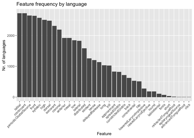
This plot shows that the features labial and continuant (i.e. the set of sounds that are not stops or affricates) are the most common in languages cross-linguistically. The feature periodic glottal source, aka voice, is third.
ggplot(cross_features, aes(reorder(x = value, -total), y = total)) +
  geom_bar(stat = "identity") +
  theme(axis.text.x = element_text(angle = 45, hjust = 1)) +
  labs(x = "Feature", y = "Nr. of languages") +
  ggtitle("Feature frequency by language")
Most languages employ the phonological feature labial to encode
contrastive sounds in their language.
Because we want to know which languages employ the phonological feature labial in our phylogenetic analysis below, we first create a table with those values.
labial_features <- features %>% filter(value == "labial")
traits <- phoible %>%
  select(InventoryID, Glottocode) %>%
  distinct()
traits <- left_join(traits, labial_features, by = c("InventoryID" = "name"))

traits <- traits %>% mutate(value = replace(value, is.na(value), "N"))
traits <- traits %>% mutate(value = replace(value, value == "labial", "Y"))

traits <- traits %>% select(-InventoryID)
traits <- traits %>% rename(taxa = Glottocode, has_labial = value)

# Remove the NA glottocodes in phoible
traits <- traits %>% filter(!is.na(taxa))

# There are a handful of dimensionality reduction results that do not agree
# tmp <- traits %>% group_by(taxa) %>% summarize(labials = paste(labial, collapse = ','))
# tmp %>% filter(grepl("T,F", labials))
# tmp %>% filter(grepl("F,T", labials))

# For now we just take the first result and discard the rest
traits <- traits %>%
  group_by(taxa) %>%
  slice_head() %>%
  ungroup()

# Sometimes... just (a)R(rgh)
traits <- as.data.frame(traits)
rownames(traits) <- NULL
rownames(traits) <- traits[, 1]First let’s have a look at data that exist for ancient and reconstructed languages. For example, we have seen that missing (bi)labials include areal features, for example, in Africa. What percentage of languages lack /p/ but contain /b/?
phoible_by_iso_with_b <- phoible %>% filter(grepl("b", Phoneme))
phoible_by_iso_with_b <- phoible_by_iso_with_b %>% filter(!(ISO6393 == "mis"))
phoible_by_iso_with_b <- phoible_by_iso_with_b %>% filter(!grepl("ɡb", Phoneme)) # Let's drop labial velars
phoible_by_iso_with_b <- phoible_by_iso_with_b %>%
  select(ISO6393) %>%
  distinct() %>%
  arrange(ISO6393)

with_p <- phoible_by_iso_with_p %>%
  select(ISO6393) %>%
  distinct()
with_p$has_p <- TRUE

with_b <- phoible_by_iso_with_b %>%
  select(ISO6393) %>%
  distinct()
with_b$has_b <- TRUE

results <- full_join(with_p, with_b)
results <- results %>% filter(is.na(has_p) & has_b)
So, roughly 6% of languages in the PHOIBLE sample contain a voiced bilabial plosive, but lack its voiceless counterpart.
nrow(results) / num_languages## [1] 0.06118547
Where are they spoken?
b_but_no_p <- phoible %>%
  filter(ISO6393 %in% results$ISO6393) %>%
  select(ISO6393, latitude, longitude, macroarea) %>%
  distinct() %>%
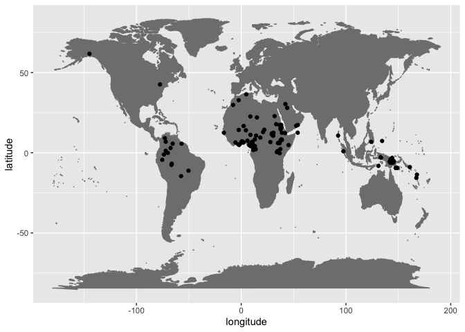
arrange(macroarea)ggplot(data = b_but_no_p, aes(x = longitude, y = latitude)) +
borders("world", colour = "gray50", fill = "gray50") +
geom_point()Mainly in Africa, in which this phenomenon has also been noted as a feature north of the equator and in the Arabian peninsula. It is also known that Arabic lost its /p/ in prehistoric times, but it is unclear whether the lack of /p/ in these areas is due to Arabic’s influence as a prestige language or whether the effect itself is even more ancient.
Hence, one interesting area to investigate the cross-linguistic frequency of labial sounds is in ancient and reconstruction languages of the world. BDPROTO is a database of phonological inventories from ancient and reconstructed languages (Marsico et al. 2018; Moran, Grossman, and Verkerk 2020). We can evaluate these (proto) languages for the presence or absence of bilabials in ancient times.
bdproto <- read_csv(url("https://raw.githubusercontent.com/bdproto/bdproto/master/bdproto.csv"))
num_languages_bdproto <- bdproto %>%
  select(BdprotoID) %>%
  distinct()
We note that by using BDPROTO phonological inventory IDs we count different reconstructions of the same proto-language in several cases and that some of the proto-languages are embedded within higher order language families, e.g. Germanic within Indo-European. For issues regarding so-called temporal bias, refer to Moran, Grossman, and Verkerk (2020) and Moran, Lester, and Grossman (2021).
bdproto <- bdproto %>% filter(!(is.na(BdprotoID)))

bdproto_with_b <- bdproto %>% filter(grepl("b", Phoneme))
bdproto_with_b <- bdproto_with_b %>% filter(!grepl("ɡb|mb", Phoneme))
bdproto_with_b %>%
  select(Phoneme) %>%
  distinct()
## # A tibble: 9 × 1
## Phoneme
## <chr>
## 1 b
## 2 bʰ
## 3 ˀb
## 4 b̥
## 5 bː
## 6 b̤ʰ
## 7 bʲ
## 8 bʷ
## 9 bʼ
bdproto_with_b <- bdproto_with_b %>%
  select(BdprotoID) %>%
  distinct() %>%
  arrange(BdprotoID)
bdproto_with_b$has_b <- TRUE

bdproto_with_p <- bdproto %>% filter(grepl("p", Phoneme))
bdproto_with_p <- bdproto_with_p %>% filter(!grepl("kp|mp", Phoneme))
bdproto_with_p %>%
  select(Phoneme) %>%
  distinct()
## # A tibble: 13 × 1
## Phoneme
## <chr>
## 1 p
## 2 pʼ
## 3 pʰ
## 4 pː
## 5 pʷ
## 6 pːʷ
## 7 pˀ
## 8 pʲ
## 9 ʰp
## 10 pl
## 11 pr
## 12 p̰
## 13 ˀp
bdproto_with_p <- bdproto_with_p %>%
  select(BdprotoID) %>%
  distinct() %>%
  arrange(BdprotoID)
bdproto_with_p$has_p <- TRUE

bdproto_results <- full_join(bdproto_with_p, bdproto_with_b)
Which ancient and reconstructed languages lack labial plosives /p/ and /b/? None.
bdproto_results %>% filter(is.na(has_p) & is.na(has_b))## # A tibble: 0 × 3
## # … with 3 variables: BdprotoID <dbl>, has_p <lgl>, has_b <lgl>
Which lack a /p/? 15 out of 253 data points, so around 8%.
bdproto_results %>% filter(is.na(has_p))## # A tibble: 19 × 3
## BdprotoID has_p has_b
## <dbl> <lgl> <lgl>
## 1 5 NA TRUE
## 2 8 NA TRUE
## 3 31 NA TRUE
## 4 71 NA TRUE
## 5 159 NA TRUE
## 6 166 NA TRUE
## 7 184 NA TRUE
## 8 185 NA TRUE
## 9 186 NA TRUE
## 10 190 NA TRUE
## 11 1014 NA TRUE
## 12 1023 NA TRUE
## 13 1025 NA TRUE
## 14 1032 NA TRUE
## 15 1039 NA TRUE
## 16 1059 NA TRUE
## 17 1081 NA TRUE
## 18 2002 NA TRUE
## 19 2015 NA TRUE
Which lack a /b/? Quite a few more – 94 out of 253 data points, so around 37%.
bdproto_results %>% filter(is.na(has_b))## # A tibble: 93 × 3
## BdprotoID has_p has_b
## <dbl> <lgl> <lgl>
## 1 10 TRUE NA
## 2 20 TRUE NA
## 3 21 TRUE NA
## 4 22 TRUE NA
## 5 23 TRUE NA
## 6 24 TRUE NA
## 7 25 TRUE NA
## 8 26 TRUE NA
## 9 27 TRUE NA
## 10 30 TRUE NA
## # … with 83 more rows
Which lack a /p/ but not /b/?
bdproto_results %>% filter(is.na(has_p) & has_b)## # A tibble: 19 × 3
## BdprotoID has_p has_b
## <dbl> <lgl> <lgl>
## 1 5 NA TRUE
## 2 8 NA TRUE
## 3 31 NA TRUE
## 4 71 NA TRUE
## 5 159 NA TRUE
## 6 166 NA TRUE
## 7 184 NA TRUE
## 8 185 NA TRUE
## 9 186 NA TRUE
## 10 190 NA TRUE
## 11 1014 NA TRUE
## 12 1023 NA TRUE
## 13 1025 NA TRUE
## 14 1032 NA TRUE
## 15 1039 NA TRUE
## 16 1059 NA TRUE
## 17 1081 NA TRUE
## 18 2002 NA TRUE
## 19 2015 NA TRUE
Which lack a /b/ but not /p/?
bdproto_results %>% filter(is.na(has_b) & has_p)## # A tibble: 93 × 3
## BdprotoID has_p has_b
## <dbl> <lgl> <lgl>
## 1 10 TRUE NA
## 2 20 TRUE NA
## 3 21 TRUE NA
## 4 22 TRUE NA
## 5 23 TRUE NA
## 6 24 TRUE NA
## 7 25 TRUE NA
## 8 26 TRUE NA
## 9 27 TRUE NA
## 10 30 TRUE NA
## # … with 83 more rows
Interestingly, no ancient or reconstructed languages in the BDPROTO lack both /p/ and /b/. And the general tendency, if either one or the other is missing, is to favor /p/.
What about bilabial fricatives. About 9 percent of the data points reported in BDPROTO have them.
bdproto_bialbials <- bdproto %>% filter(grepl("ɸ|β", Phoneme))
lgs_with_bdproto_bialbials <- bdproto_bialbials %>%
  select(BdprotoID) %>%
  distinct()
nrow(lgs_with_bdproto_bialbials) / nrow(bdproto %>% select(BdprotoID) %>% distinct())
## [1] 0.0858209
How many data points do not have Glottocodes – a marker of how many languages / dialects are reported in BDPROTO – 214 out of 272.
nrow(bdproto %>% select(BdprotoID) %>% distinct())## [1] 268
nrow(bdproto %>% select(Glottocode) %>% filter(!is.na(Glottocode)) %>% distinct())## [1] 212
Does the frequency of the presence of bilabial fricatives change if we subset the data on Glottocodes? It actually goes up to about 10%.
bdproto_bialbials <- bdproto %>%
  filter(!is.na(Glottocode)) %>%
  filter(grepl("ɸ|β", Phoneme))
lgs_with_bdproto_bialbials <- bdproto_bialbials %>%
  select(Glottocode) %>%
  distinct()
nrow(lgs_with_bdproto_bialbials) / nrow(bdproto %>% select(Glottocode) %>% filter(!is.na(Glottocode)) %>% distinct())
## [1] 0.09433962
When compared to PHOIBLE is this prevalence of languages with contrastive (or reconstructed) bilabial fricatives greater or less today than in the past? We might expect the percentage to go down, as sounds shift to, for example, labiodentals (Blasi et al. 2019; Moran, Lester, and Grossman 2021), which have a greater intensity of noise and greater amplitude. (Maddieson (2005) notes, however, that the differences between bilabial fricatives and labiodental fricatives in the few languages that contrast them may not be subtle to speakers of those languages.)
Let’s calculate phoible by ISO 639-3 language codes. PHOIBLE actually has a higher percentage of bilabial fricatives than in the BDPROTO study at nearly 17%.
phoible_bialbials <- phoible %>%
  filter(!is.na(ISO6393)) %>%
  filter(grepl("ɸ|β", Phoneme))
lgs_with_phoible_bialbials <- phoible_bialbials %>%
  select(ISO6393) %>%
  distinct()
nrow(lgs_with_phoible_bialbials) / nrow(phoible %>% select(ISO6393) %>% filter(!is.na(ISO6393)) %>% distinct())
## [1] 0.167304
Next we undertake a phylogenetic analysis of the feature labial. That is, we would like to know whether within certain language families (for which there exits high resolution phylogenies) if the feature labial is present or not present during the evolution of languages within particular families. However, what we find is that the feature labial is present throughout all of the daughter languages for which we have data and high resolution phylogenies.
We define some convenience functions for pruning the phylogenies with the PHOIBLE data.
PruneTraits <- function(traits, tip.labels) {
  traits.cut <- subset(traits, traits$taxa %in% tip.labels)
  return(traits.cut)
}

PruneSummaryTree <- function(nexus.file, codes, which = c("LanguageName", "ISO", "Glottocode")) {
  # Trees have tip labels like "Ache<ache1246|guq>" with language name and Glottolog codes. Take Glottolog code. Return tree.
  tree <- read.nexus(nexus.file)
  switch(which,
    Glottocode = {
      tree$tip.label <- gsub("(.*)(<)(.*)(\\|)(.*)(>)", "\\3", tree$tip.label)
    },
    ISO = {
      tree$tip.label <- gsub("(.*)(<)(.*)(\\|)(.*)(>)", "\\5", tree$tip.label)
    },
    LanguageName = {
      tree$tip.label <- gsub("(.*)(<)(.*)(\\|)(.*)(>)", "\\1", tree$tip.label)
    }
  )
  # Drop tips missing in traits
  tree <- drop.tip(tree, setdiff(tree$tip.label, codes))
  # Remove any remaining duplicates.
  if (any(duplicated(tree$tip.label))) {
    index <- which(duplicated(tree$tip.label))
    tree$tip.label[index] <- "remove"
    tree <- drop.tip(tree, "remove")
  }
  return(tree)
}
First we prune the Indo-European phylogeny as published by (Chang et al. 2015), which is available via D-PLACE (Kirby et al. 2016).
# Tree paths
tree <- "trees/ie-c-tree.nex"
pr_sum_tree <- PruneSummaryTree(tree, traits$taxa, "Glottocode")

# Prune the traits data to match the tree tips for analysis
data <- PruneTraits(traits, pr_sum_tree$tip.label)

# Combine them into a list of R data objects for analysis with the BT3 wrapper
pr_sum_tree <- list(data = data, tree = pr_sum_tree)
Here is a convenience function for plotting the phylogeny together with the presence of absence of a discrete variable.
# Define color schema
color.scheme <- c("blue", "red")
names(color.scheme) <- c("Y", "N")

# Function to reverse time in the plot
reverse.time <- function(p) {
  p$data$x <- p$data$x - max(p$data$x)
  return(p)
}

# Create tree and heatmap figure
plot.tree <- function(pr_sum_tree_plot, features_plot) {
  gheatmap(pr_sum_tree_plot, features_plot,
    colnames_position = "top", color = "black",
    colnames_offset_y = 0.1, font.size = 2.5,
    width = 0.4, offset = 8
  ) +
    scale_fill_manual(name = "", values = color.scheme) +
    scale_x_continuous(breaks = c(-6000, -4000, -2000, 0)) +
    scale_y_continuous(expand = c(-0.01, 1)) +
    theme_tree2(axis.text.x = element_text(size = 8)) +
    theme(
      legend.position = "none",
      axis.ticks = element_line(color = "grey")
    )
}
Next we plot the presence of absence of each trait (has or does not have labial as a contrastive phonological feature) on the phylogeny.
traits.print <- pr_sum_tree$data %>% select(has_labial)

p <- reverse.time(ggtree(pr_sum_tree$tree, ladderize = T, right = T)) +
  geom_tiplab(align = T, linesize = .1, size = 2)
plot.tree(p, traits.print)
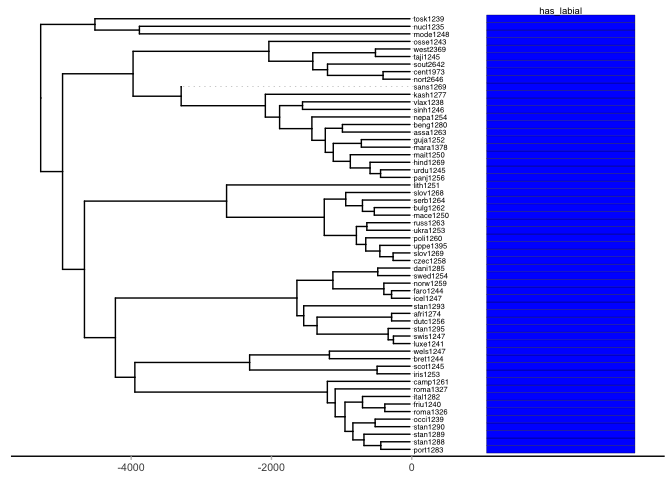
What we find is that within the Indo-European phylogeny the feature labial is present in all daughter nodes of the family tree (which has been pruned to the languages that we have information about in PHOIBLE). Thus, we cannot generate for example a stochastic character mapping on the Indo-European tree because there is only one dimension, i.e., one categorical value for the input to the model, and that value is always present.
We can only assume that either all languages innovated a labial contrast and the root node (the proto-language) did not have labial contrastive segments – or the that the proto-language used the labial feature and all languages have kept that feature through time. Given the cross-linguistic frequency of contrastive labial segments in phonological inventories and the extreme rarity in which they are absent in a handful of languages in the PHOIBLE sample, we assume that labial has long been a feature of spoken languages.
Next we prune the Sino-Tibetan phylogeny as published by M. Zhang et al. (2019) and also available via D-PLACE (Kirby et al. 2016).
# Tree paths
tree <- "trees/sinotibetan-z-tree.nex"
pr_sum_tree <- PruneSummaryTree(tree, traits$taxa, "Glottocode")

# Prune the traits data to match the tree tips for analysis
data <- PruneTraits(traits, pr_sum_tree$tip.label)

# Combine them into a list of R data objects for analysis with the BT3 wrapper
pr_sum_tree <- list(data = data, tree = pr_sum_tree)
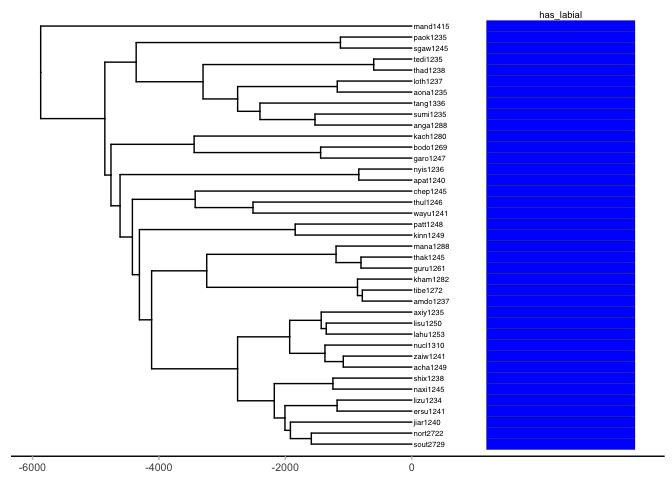
We plot at the distribution of the feature labial in Sino-Tibetan. Again, we see that the feature labial is present in all daughter nodes of the phylogeny, leading us to the same conclusion as in Indo-European – labial is a (near) universal phonologically contrastive feature used by spoken languages.
traits.print <- pr_sum_tree$data %>% select(has_labial)

p <- reverse.time(ggtree(pr_sum_tree$tree, ladderize = T, right = T)) +
  geom_tiplab(align = T, linesize = .1, size = 2)
plot.tree(p, traits.print)Abbott, Clifford. 2006. Oneida Teaching Grammar. University of Wisconsin – Green Bay. https://www.uwgb.edu/UWGBCMS/media/Oneida-Language/files/teaching-grammar-revised4.pdf.
Blasi, Damián E., Steven Moran, Scott R. Moisik, Paul Widmer, Dan Dediu, and Balthasar Bickel. 2019. “Human Sound Systems Are Shaped by Post-Neolithic Changes in Bite Configuration.” Science 363 (6432). https://doi.org/10.1126/science.aav3218.
Chang, Will, Chundra Cathcart, David Hall, and Andrew Garrett. 2015. “Ancestry-Constrained Phylogenetic Analysis Supports Indo-European Steppe Hypothesis.” Language 91: 194–244. https://doi.org/10.1353/lan.2015.0005.
Clements, G. N., and Annie Rialland. 2008. “Africa as a Phonological Area.” In A Linguistic Geography of Africa, edited by Bernd Heine and Derek Nurse, 36–85. Cambridge: Cambridge University Press.
Grossman, Eitan, Elad Eisen, Dmitry Nikolaev, and Steven Moran. 2020. “SegBo: A Database of Borrowed Sounds in the World’s Languages.” In Proceedings of the 12th Language Resources and Evaluation Conference, 5316–22. Marseille, France: European Language Resources Association. https://www.aclweb.org/anthology/2020.lrec-1.654.
Hammarström, Harald, Robert Forkel, Martin Haspelmath, and Sebastian Bank. 2020. Glottolog 4.2.1. Jena: Max Planck Institute for the Science of Human History; Max Planck Institute for the Science of Human History. https://doi.org/10.5281/zenodo.3754591.
Houis, Maurice. 1974. “A Propos de /p/.” Afrique Et Langage 1: 35–38.
Kirby, Kathryn R., Russell D. Gray, Simon J. Greenhill, Fiona M. Jordan, Stephanie Gomes-Ng, Hans-Jörg Bibiko, Damián E. Blasi, et al. 2016. “D-PLACE: A Global Database of Cultural, Linguistic and Environmental Diversity.” PLoS ONE 11 (7): e0158391.
Lounsbury, Floyd G. 1953. Oneida Verb Morphology. Yale University Publications in Anthropology. New Haven: Yale University Press.
Maddieson, Ian. 1984. Patterns of Sounds. Cambridge: Cambridge University Press.
———. 2005. “Bilabial and Labio-Dental Fricatives in Ewe.” UC Berkeley Phonology Lab Annual Report 1 (1). https://escholarship.org/uc/item/4r49g6qx.
Marsico, Egidio, Sebastien Flavier, Annemarie Verkerk, and Steven Moran. 2018. “BDPROTO: A Database of Phonological Inventories from Ancient and Reconstructed Languages.” In Proceedings of the 11th International Conference on Language Resources and Evaluation (LREC 2018).
Michelson, Karin. 1990. “The Oneida Lexicon.” In Proceedings of the Sixteenth Annual Meeting of the Berkeley Linguistics Society: Special Session on General Topics in American Indian, 16:73–84. 2.
Moran, Steven, Eitan Grossman, and Annemarie Verkerk. 2020. “Investigating Diachronic Trends in Phonological Inventories Using BDPROTO.” Language Resources and Evaluation. https://doi.org/https://doi.org/10.1007/s10579-019-09483-3.
Moran, Steven, Nicholas A. Lester, and Eitan Grossman. 2021. “Inferring Recent Evolutionary Changes in Speech Sounds.” Philosophical Transactions of the Royal Society B: Biological Sciences 376 (20200198). https://doi.org/https://doi.org/10.1098/rstb.2020.0198.
Moran, Steven, and Daniel McCloy, eds. 2019. PHOIBLE 2.0. Jena: Max Planck Institute for the Science of Human History. https://phoible.org/.
R Core Team. 2021. R: A Language and Environment for Statistical Computing. Vienna, Austria: R Foundation for Statistical Computing. https://www.R-project.org/.
Revell, Liam J. 2012. “Phytools: An r Package for Phylogenetic Comparative Biology (and Other Things).” Methods in Ecology and Evolution 3: 217–23.
Wickham, Hadley. 2011. “Testthat: Get Started with Testing.” The R Journal 3: 5–10. https://journal.r-project.org/archive/2011-1/RJournal_2011-1_Wickham.pdf.
Wickham, Hadley, Mara Averick, Jennifer Bryan, Winston Chang, Lucy D’Agostino McGowan, Romain François, Garrett Grolemund, et al. 2019. “Welcome to the tidyverse.” Journal of Open Source Software 4 (43): 1686. https://doi.org/10.21105/joss.01686.
Xie, Yihui. 2021. Knitr: A General-Purpose Package for Dynamic Report Generation in r. https://yihui.org/knitr/.
Yu, Guangchuang. 2020. “Using Ggtree to Visualize Data on Tree‐Like Structures.” Curr. Protoc. Bioinformatics 69 (1). https://doi.org/10.1002/cpbi.96.
Zhang, Jinlong. 2017. Phylotools: Phylogenetic Tools for Eco-Phylogenetics. https://CRAN.R-project.org/package=phylotools.
Zhang, Menghan, Shi Yan, Wuyun Pan, and Li Jin. 2019. “Phylogenetic Evidence for Sino-Tibetan Origin in Northern China in the Late Neolithic.” Nature 569 (7754): 112–15. https://doi.org/10.1038/s41586-019-1153-z.

