| title | author | date | output | ||||||||
|---|---|---|---|---|---|---|---|---|---|---|---|
Olivia R package |
Tamar Sofer & Nuzulul Kurniansyah |
2/18/2021 |
|
Here we demonstrate how to perform association analyses of continuous phenotypes using the Olivia package with RNA-seq data based on the pipeline proposed in the manuscript Benchmarking Association Analyses of Continuous Exposures with RNA-seq in Observational Studieshttps://academic.oup.com/bib/advance-article-abstract/doi/10.1093/bib/bbab194/6278609.
Click here for instructions on using Olivia as a Shiny app.
To install, open R and type:
library("devtools")
install_github("nkurniansyah/Olivia")
library(Olivia)
Olivia requires external packages from CRAN (dplyr, ggplot2, tableone, reshape, and ggrepel) and Bioconductor(qvalue)
install.packages("dplyr")Load packages
library(dplyr)
library(ggplot2)
library(reshape2)
library(tableone)
library(ggrepel)
library(EnsDb.Hsapiens.v86)First we load the transcripts. The transcripts were obtained from https://www.ncbi.nlm.nih.gov/geo/query/acc.cgi?acc=GSE151243. Note: we reformatted the transcript matrix into desired form and embedded them into the Olivia package.
data(rnaseq_count_matrix)
rnaseq_count_matrix[1:5,1:5]
## 10L_S26_L006_R1_001 10N_S15_L003_R1_001 11L_S35_L007_R1_001 11N_S25_L005_R1_001 12L_S14_L003_R1_001
## ENSG00000000003 446 644 525 701 572
## ENSG00000000005 5 19 2 64 25
## ENSG00000000419 883 1058 609 547 576
## ENSG00000000457 790 1009 619 887 650
## ENSG00000000460 206 289 272 214 334
We simulated in advance a data.frame of phenotypes.
data(phenotype)
head(phenotype)
## Age Sex Trait.1 Trait.2 Race
## 10L_S26_L006_R1_001 18 1 16.06608 15.58321 White
## 10N_S15_L003_R1_001 19 0 21.20045 20.61345 Asian
## 11L_S35_L007_R1_001 20 0 14.44867 13.88567 Black
## 11N_S25_L005_R1_001 21 0 35.89606 34.84859 White
## 12L_S14_L003_R1_001 22 1 24.09078 24.42536 Asian
## 12N_S27_L006_R1_001 21 1 29.61045 26.62854 Asian
We create a table summarizing the phenotypes.
summary_phen<- summarize_phenotypes(pheno = phenotype,
                                    categorical_variables = c("Sex"),
                                    numeric_variables = c("Age","Trait.1","Trait.2"),
                                    strata = "Race")
## Generate summary of phenotype using Sex Age Trait.1 Trait.2
summary_phen## Stratified by Race
## Asian Black White
## n 11 12 17
## Sex = 1 (%) 6 (54.5) 4 (33.3) 10 (58.8)
## Age (mean (SD)) 37.00 (13.67) 35.83 (11.14) 37.82 (11.41)
## Trait.1 (mean (SD)) 26.62 (5.17) 24.36 (8.88) 25.40 (8.04)
## Trait.2 (mean (SD)) 26.14 (4.97) 24.18 (8.77) 25.89 (8.25)
We define the trait of interest to study as an exposure associated with genes. The trait/phenotype has to correspond to a column name in the phenotype data.frame.
trait <- "Trait.1"We will adjust our analysis to the simulated covariates Age and Sex. The covariates have to correspond to column names in the phenotype data.frame. In the analysis, we will use a string defining the regression model (just the covariates part of it), so we define it here:
covariates_string <- "Age + Sex"Note that we can also define the string to be "Age + as.factor(Sex)", or use interaction terms, like one would use in regression functions in R.
Match the (simulated) individuals between the phenotype and the RNA-seq count matrix. Make sure the there are matching IDs.
IDs_both <- intersect(rownames(phenotype), colnames(rnaseq_count_matrix))
rnaseq_matrix <- rnaseq_count_matrix[, IDs_both]
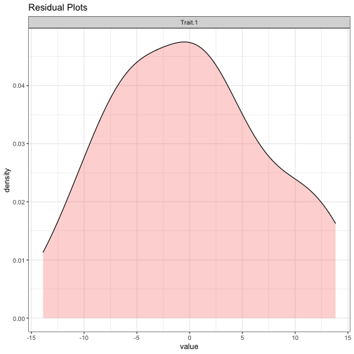
phenotypes <- phenotype[match(IDs_both,rownames(phenotype)),]After defining the trait of interest and covariates to adjust to the model, it is helpful to look at the trait's residual distribution.
resid_plot<- residual_plot(pheno = phenotype,
                           traits = trait,
                           covariates_string = covariates_string)
## Generate residual of Trait.1...
## Generate the residual plot...
resid_plotHere, the residuals' distribution has short tails.
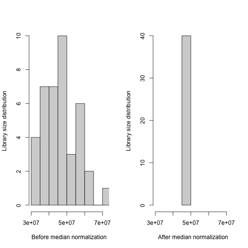
We use median normalization in Olivia to reduce package dependencies. However, users can use different normalization method using different packages, for example: estimateSizeFator(DESeq2) or TMM(edgeR). There are no downstream differences in how the methods are applied once the data is normalized.
After median normalization, the sum of the gene expression values over all transcripts is the same across individuals.
median_norm <- median_normalization(rnaseq_matrix)

xrange <- range(colSums(rnaseq_matrix))
par(mfrow = c(1,2))
hist(colSums(rnaseq_matrix),
     xlim = xrange,
     main = "",
     xlab = "Before median normalization",
     ylab = "Library size distribution")
hist(colSums(median_norm),
     xlim = xrange,
     main = "",
     xlab = "After median normalization",
ylab = "Library size distribution")Remove lowly expressed genes
clean_count_matrix <- apply_filters(count_matrix = median_norm,
                                    median_min = 1,
                                    expression_sum_min = 10,
                                    max_min = 10,
                                    range_min = 5,
                                    prop_zero_max = 0.5)
## applying filters on a transcript count matrix of 58051 transcripts, across 40 individuals
## Computing transtripts characteristics...
## Appying filters...
## There are 23987 transcripts with median
##                   value lower than 1
## There are 14190 transcripts with expression sum
##                   value lower than 10
## There are 22297 transcripts with maximum expression
##                   value lower than 10
## There are 17188 transcripts with maximum
##                   expression range value lower than 5
## There are 21923 transcripts with propotion
##                   of zero counts higher than 0.5
## Removing 24834 unique transcripts not passing requested filters
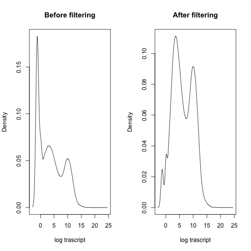
After filtering genes, there are 33217 remaining for differential expression analysis. The plot below illustrates the proportion of transcripts/genes in the “12N_S27_L006_R1_001” sample (selected randomly) before and after filtering.
par(mfrow=c(1,2))
plot(density(log_replace_half_min(median_norm)[,"12N_S27_L006_R1_001"]),
     main="Before filtering", xlab="log trascript")
plot(density(log_replace_half_min(clean_count_matrix)[,"12N_S27_L006_R1_001"]),
     main="After filtering", xlab="log trascript")
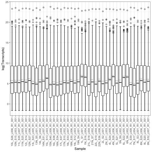
The figure below shows the distribution of transcript expressions (counts) in the sample in boxplots after filtering and after log transformation.
log_counts<- log_replace_half_min(clean_count_matrix)
log_counts<-melt(log_counts)

box_plot<- ggplot(log_counts, aes(x = Var2, y = value)) +
                  stat_boxplot(aes(Var2, value),
                  geom='errorbar', linetype=1, width=0.5)+
                  xlab("Sample")+
                  ylab("log(Transcripts)")+
                  geom_boxplot( aes(Var2, value),outlier.shape=1)+
                  stat_summary(fun = mean, geom = "errorbar",
                                aes(ymax = ..y.., ymin = ..y..),
                                width = .75, linetype = "dotted") +
                 theme_bw()+
                 theme(axis.text.x = element_text(angle = 90, vjust = 0.5, hjust=1))

box_plotWe show how we perform differential expression analysis (Transcriptome-wide association study) on all transcripts using empirical p-value (quantile empirical p-values). To generate p-values under the null, we create a residual permuted trait 100 times, perform differential expression analysis, and use the resulting p-values as our null p-values. However, users also can implement Storey empirical p-value (as these are referred to in the manuscript) using test statistics.
set.seed(12)

quantile_emp_trascript<-lm_count_mat_emp_pval(clean_count_matrix,
                                              pheno=phenotypes,
                                              trait=trait,
                                              covariates_string=covariates_string,
                                              n_permute=100,
                                              log_transform = "log_replace_half_min",
                                              outcome_type ="continuous",
                                              gene_IDs=NULL)
## Performing residual permutation to generate permuted trait...
## performing differential expression analysis on 100 permuted traits
## Computing quantile empirical p-values
We do not implement the annotation feature into the Olvia package, to limit chances to run into compatibility issues as packages update. We here demonstrate how to create a function to add an annotation in a transcriptome-wide association study. We use EnsDb.Hsapiens.v86
add_annotation<-function(deg_res){

   gene_symbol<- select(EnsDb.Hsapiens.v86,
                        keys =as.character(deg_res$geneID) ,
                        keytype = "GENEID",
                        columns = c("GENEID", "GENENAME"))

   colnames(gene_symbol)<- c("geneID","geneName")

   annot_deg<-left_join(deg_res,gene_symbol, by="geneID")
   annot_deg<- annot_deg %>% dplyr::rename(IDs=geneID,
                                           geneID= geneName)
   return(annot_deg)

}
quantile_emp_trascript <- add_annotation(quantile_emp_trascript)
head(quantile_emp_trascript)## IDs adjLogFC se t_stat t_stat_df p_value fdr_bh emp_pvals bh_emp_pvals geneID
## 1 ENSG00000000003 0.017357492 0.010049207 1.7272499 36 9.269483e-02 0.369384496 1.019728e-01 0.40635317 TSPAN6
## 2 ENSG00000000005 0.169923122 0.024726980 6.8719723 36 4.835620e-08 0.001606248 1.505253e-07 0.00250000 TNMD
## 3 ENSG00000000419 0.002683873 0.014082843 0.1905775 36 8.499273e-01 0.954520056 8.552118e-01 0.96045199 DPM1
## 4 ENSG00000000457 0.006484793 0.009770087 0.6637395 36 5.110857e-01 0.812322708 5.245516e-01 0.83372554 SCYL3
## 5 ENSG00000000460 -0.017100775 0.012268212 -1.3939093 36 1.718902e-01 0.505504776 1.841322e-01 0.54149836 C1orf112
## 6 ENSG00000000938 -0.074471226 0.019795282 -3.7620695 36 5.999232e-04 0.030517578 8.275883e-04 0.04205167 FGR
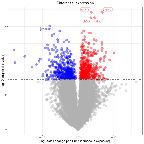
Now, we can obtain significant genes (the genes which have bh_emp_pvals < 0.05)
tophits <- quantile_emp_trascript[which(quantile_emp_trascript$bh_emp_pvals< 0.05),]
head(tophits)
## IDs adjLogFC se t_stat t_stat_df p_value fdr_bh emp_pvals bh_emp_pvals geneID
## 2 ENSG00000000005 0.16992312 0.024726980 6.871972 36 4.835620e-08 0.001606248 1.505253e-07 0.00250000 TNMD
## 6 ENSG00000000938 -0.07447123 0.019795282 -3.762069 36 5.999232e-04 0.030517578 8.275883e-04 0.04205167 FGR
## 12 ENSG00000001461 0.03820379 0.009127139 4.185735 36 1.747104e-04 0.023064772 2.146491e-04 0.02840637 NIPAL3
## 107 ENSG00000005844 -0.07031756 0.017600485 -3.995206 36 3.057323e-04 0.025733375 3.991932e-04 0.03382278 ITGAL
## 116 ENSG00000006016 0.08467400 0.020904358 4.050543 36 2.600651e-04 0.024333821 3.287473e-04 0.03076056 CRLF1
## 123 ENSG00000006118 -0.08471630 0.021090465 -4.016806 36 2.870448e-04 0.025225994 3.730018e-04 0.03271768 TMEM132A
After completing the transcriptome-wide association study, now we can visualize up-regulated and down-regulated genes using a volcano plot.
volcano <- volcano_plot(deg_res = quantile_emp_trascript,
                        significant_threshold = 0.05 )
## Generate volcano plot..
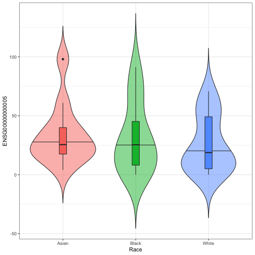
volcanoLooking at the results, we may want to see how a transcript of interest (e.g. the most significantly-associated gene) distributes across population strata. We here visualize this using violin plots. The row names in the matrix of transcript counts and in the phenotype matrix have to match.
top_gene<- "ENSG00000000005"
violin_plot(pheno = phenotypes,
            strata = "Race",
            norm_count_matrix  = clean_count_matrix,
            selected_transcript = top_gene)
## Generate violin plot for ENSG00000000005 and stratified by Race
When testing only a handful of genes, we may not want to perform a transcriptome-wide association analysis. Therefore, empirical p-values using the quantile or Storey's approach cannot be computed (not enough tests to generate the null distribution). Instead, we permute specific genes many times. Here we show how to perform differential expression analysis on selected transcripts when computing a permutation p-value for each gene based on permutations for this gene only. We suggest running 100000 permutations, but more permutation are needed if higher precision in p-value computation is needed.
set.seed(12)

gene_names<-sample(rownames(clean_count_matrix),3)

perm_res<- lm_count_mat_perm_pval(count_matrix=clean_count_matrix,
                                  pheno=phenotypes,
                                  trait=trait,
                                  covariates_string=covariates_string,
                                  n_permute=100000,
                                  gene_IDs=gene_names,
                                  seed = NULL,
                                  log_transform = "log_replace_half_min",
                                  outcome_type ="continuous")
## Filtering count_matrix to genes : ENSG00000211888 ENSG00000100416 ENSG00000039650
## Performing residual permutation to generate permuted trait...
perm_res<-add_annotation(perm_res)

head(perm_res)
## IDs adjLogFC se t_stat t_stat_df p_value perm_pval geneID
## 1 ENSG00000211888 -0.112482869 0.03583958 -3.138510 36 0.003381306 0.00335 TRAJ1
## 2 ENSG00000100416 -0.009668082 0.01282077 -0.754095 36 0.455696677 0.45678 TRMU
## 3 ENSG00000039650 -0.026389697 0.01027976 -2.567152 36 0.014554899 0.01258 PNKP
We show how we perform differential expression analysis on all transcripts using emprical p-value(quantile empirical p-values) when testing association using multiple exposure at the same time.
set.seed(12)

quantile_emp_multi<-lm_mult_count_mat_emp_pval(clean_count_matrix,
                                               pheno=phenotypes,
                                               traits=c("Trait.1","Trait.2") ,
                                               covariates_string=covariates_string,
                                               n_permute=100,
                                               gene_IDs=NULL,
                                               log_transform = "log_replace_half_min",
                                               outcome_type="continuous")
## Performing residual permutation to generate permuted trait...
## performing differential expression analysis on 100 permuted traits
## Computing quantile empirical p-values
quantile_emp_multi<-add_annotation(quantile_emp_multi)
head(quantile_emp_multi)
## IDs adjLogFC_Trait.1 adjLogFC_Trait.2 chisq_stat chisq_stat_df p_value fdr_bh emp_pvals bh_emp_pvals
## 1 ENSG00000000003 -0.10675797 0.12623124 5.9029877 2 5.226158e-02 2.498162e-01 7.272601e-02 0.3476385
## 2 ENSG00000000005 0.41402432 -0.24826235 49.8933559 2 1.464858e-11 4.865818e-07 1.505253e-07 0.0050000
## 3 ENSG00000000419 -0.15522792 0.16060370 2.2915987 2 3.179696e-01 6.034386e-01 3.439989e-01 0.6528065
## 4 ENSG00000000457 -0.03785637 0.04509704 0.7829863 2 6.760467e-01 8.458419e-01 6.945609e-01 0.8690008
## 5 ENSG00000000460 -0.11979076 0.10444052 3.1761359 2 2.043200e-01 4.921484e-01 2.311103e-01 0.5566630
## 6 ENSG00000000938 -0.05065862 -0.02421854 13.7940006 2 1.010813e-03 3.432332e-02 3.668001e-03 0.1243249
## geneID
## 1 TSPAN6
## 2 TNMD
## 3 DPM1
## 4 SCYL3
## 5 C1orf112
## 6 FGR
Now, we can identify significantly-associated genes based on transcriptome-wide associations using multiple exposures (the genes which have bh_emp_pvals < 0.05)
top_emp_multi<-quantile_emp_multi[quantile_emp_multi$bh_emp_pvals< 0.05,]
rownames(top_emp_multi)<-NULL

head(top_emp_multi)
## IDs adjLogFC_Trait.1 adjLogFC_Trait.2 chisq_stat chisq_stat_df p_value fdr_bh emp_pvals bh_emp_pvals geneID
## 1 ENSG00000000005 0.4140243 -0.248262354 49.89336 2 1.464858e-11 4.865818e-07 1.505253e-07 0.00500000 TNMD
## 2 ENSG00000144821 0.1005357 -0.008144529 39.42639 2 2.745790e-09 4.560345e-05 1.204203e-06 0.02000000 MYH15
## 3 ENSG00000197766 0.2948484 -0.181672393 36.53264 2 1.166911e-08 1.292043e-04 3.311557e-06 0.03666667 CFD
Olivia is available as a Shiny app. This app will run locally on your computer using gist.github.com to avoid potential memory problems when users try to run an analysis using large samples and transcripts/gene counts.
To run Olivia's shiny app, users need to have R/4.0.0 or above installed. Also, users need to install few R packages and load them before running the app.
You can download the example files from the tutorial on the Shiny app. Alternatively, you can install the Olivia R package, and save the example files as follows:
library(Olivia)
write.table(get(data("rnaseq_count_matrix")), file = "rnaseq_count_matrix.txt", quote = FALSE)
write.csv(get(data("phenotype")), file = "phenotypes.csv")
Please run the R code below before every use of the Olivia Shiny app.
# CRAN
install_cran_package <- function(pkg){
  new.pkg <- pkg[!(pkg %in% installed.packages()[, "Package"])]
  if (length(new.pkg))
    install.packages(new.pkg, dependencies = TRUE)
  sapply(pkg, library, character.only = TRUE)
}

list_packages_cran <- c("shiny","progress","shinyjs","shinythemes","scales",
                      "kableExtra","gridExtra","shinyFiles","DT","grid","data.table",
                      "plyr","tableone","reshape","BiocManager","ggrepel","dplyr","tidyverse")

install_cran_package(list_packages_cran)


# Bioconductor
install_bioconductor_package <- function(pkg){
  new.pkg <- pkg[!(pkg %in% installed.packages()[, "Package"])]
  if (length(new.pkg))
    BiocManager::install(new.pkg, dependencies = TRUE)
  sapply(pkg, library, character.only = TRUE)
}

list_packages_bioconductor <- c("EnsDb.Hsapiens.v86","fgsea")

install_bioconductor_package(list_packages_bioconductor)


# Run shiny:

shiny::runGist("ca33e0b4099ef0ca6330740a6b98be83")
