The goal of the agreement package is to calculate estimates of
inter-rater agreement and reliability using generalized formulas that
accommodate different designs (e.g., crossed or uncrossed), missing
data, and ordered or unordered categories. The package includes
generalized functions for all major chance-adjusted indexes of
categorical agreement (i.e., α, γ, Ir2, κ, π, and S) as well as all
major intraclass correlation coefficients (i.e., one-way and two-way
models, agreement and consistency types, and single measure and average
measure units). Estimates include bootstrap resampling distributions,
confidence intervals, and custom tidying and plotting functions.
You can install the development version from GitHub with:
# install.packages("devtools")
devtools::install_github("jmgirard/agreement")Calculate chance-adjusted indexes of categorical agreement for unordered categories
library(agreement)
# Load dataset with 4 raters assigning 12 objects to 5 unordered categories
data(unordered)
print(unordered)
#> # A tibble: 48 x 3
#>    Object Rater Score
#>     <int> <chr> <chr>
#>  1      1 R1    a
#>  2      1 R2    a
#>  3      1 R3    <NA>
#>  4      1 R4    a
#>  5      2 R1    b
#>  6      2 R2    b
#>  7      2 R3    c
#>  8      2 R4    b
#>  9      3 R1    c
#> 10      3 R2    c
#> # ... with 38 more rows
# Calculate all chance-adjusted indexes for unordered categories
results1 <- cat_adjusted(unordered)
#> Warning in cat_adjusted(unordered): With a small number of objects, bootstrap
#> confidence intervals may not be stable.
summary(results1, ci = TRUE, type = "perc")
#>
#> Call:
#> cat_adjusted(.data = unordered)
#>
#> Objects = 12
#> Raters = 4
#> Categories = {a, b, c, d, e}
#> Weighting = identity
#>
#> Chance-Adjusted Categorical Agreement with Bootstrapped CIs
#>
#> Observed Expected Adjusted lower upper
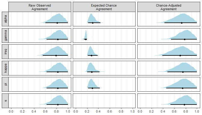
#> alpha 0.805 0.240 0.743 0.425 1
#> gamma 0.818 0.190 0.775 0.541 1
#> irsq 0.782 0.233 0.716 0.387 1
#> kappa 0.818 0.233 0.763 0.479 1
#> pi 0.818 0.239 0.761 0.453 1
#> s 0.818 0.200 0.773 0.531 1# Transform results into a tidy data frame
tidy(results1, type = "perc")
#> # A tibble: 18 x 6
#> approach weighting term estimate lower upper
#> <chr> <chr> <chr> <dbl> <dbl> <dbl>
#> 1 alpha identity Observed 0.805 0.600 1
#> 2 gamma identity Observed 0.818 0.216 0.436
#> 3 irsq identity Observed 0.782 0.425 1
#> 4 kappa identity Observed 0.818 0.625 1
#> 5 pi identity Observed 0.818 0.144 0.196
#> 6 s identity Observed 0.818 0.541 1
#> 7 alpha identity Expected 0.24 0.553 1
#> 8 gamma identity Expected 0.190 0.214 0.387
#> 9 irsq identity Expected 0.233 0.387 1
#> 10 kappa identity Expected 0.233 0.625 1
#> 11 pi identity Expected 0.239 0.202 0.421
#> 12 s identity Expected 0.2 0.479 1
#> 13 alpha identity Adjusted 0.743 0.625 1
#> 14 gamma identity Adjusted 0.775 0.218 0.424
#> 15 irsq identity Adjusted 0.716 0.453 1
#> 16 kappa identity Adjusted 0.763 0.625 1
#> 17 pi identity Adjusted 0.761 NA NA
#> 18 s identity Adjusted 0.773 0.531 1# Plot the bootstrap resampling distributions with confidence intervals
plot(results1)
#> Warning: Computation failed in `stat_sample_slabinterval()`:
#> need at least two non-NA values to interpolateCalculate chance-adjusted indexes of categorical agreement for ordered categories
# Load dataset with 5 raters assigning 20 objects to 4 ordered categories
data(ordered)
print(ordered)
#> # A tibble: 100 x 3
#>    Object Rater Score
#>     <int> <chr> <dbl>
#>  1      1 R1        1
#>  2      1 R2        1
#>  3      1 R3        2
#>  4      1 R4       NA
#>  5      1 R5        2
#>  6      2 R1        1
#>  7      2 R2        1
#>  8      2 R3        0
#>  9      2 R4        1
#> 10      2 R5       NA
#> # ... with 90 more rows
# Calculate all chance-adjusted indexes for ordered categories (linear weights)
results2 <- cat_adjusted(ordered, weighting = "linear")
summary(results2, ci = TRUE, type = "perc")
#>
#> Call:
#> cat_adjusted(.data = ordered, weighting = "linear")
#>
#> Objects = 20
#> Raters = 5
#> Categories = {0, 1, 2, 3}
#> Weighting = linear
#>
#> Chance-Adjusted Categorical Agreement with Bootstrapped CIs
#>
#> Observed Expected Adjusted lower upper
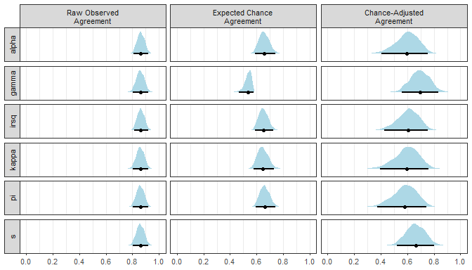
#> alpha 0.864 0.643 0.618 0.403 0.754
#> gamma 0.859 0.553 0.686 0.557 0.835
#> irsq 0.864 0.638 0.624 0.427 0.756
#> kappa 0.859 0.636 0.614 0.394 0.762
#> pi 0.859 0.648 0.601 0.375 0.747
#> s 0.859 0.583 0.663 0.523 0.803tidy(results2, type = "perc")
#> # A tibble: 18 x 6
#> approach weighting term estimate lower upper
#> <chr> <chr> <chr> <dbl> <dbl> <dbl>
#> 1 alpha linear Observed 0.864 0.809 0.919
#> 2 gamma linear Observed 0.859 0.587 0.740
#> 3 irsq linear Observed 0.864 0.403 0.754
#> 4 kappa linear Observed 0.859 0.801 0.918
#> 5 pi linear Observed 0.859 0.467 0.575
#> 6 s linear Observed 0.859 0.557 0.835
#> 7 alpha linear Expected 0.643 0.811 0.919
#> 8 gamma linear Expected 0.553 0.586 0.726
#> 9 irsq linear Expected 0.638 0.427 0.756
#> 10 kappa linear Expected 0.636 0.801 0.918
#> 11 pi linear Expected 0.648 0.576 0.732
#> 12 s linear Expected 0.583 0.394 0.762
#> 13 alpha linear Adjusted 0.618 0.801 0.918
#> 14 gamma linear Adjusted 0.686 0.592 0.741
#> 15 irsq linear Adjusted 0.624 0.375 0.747
#> 16 kappa linear Adjusted 0.614 0.801 0.918
#> 17 pi linear Adjusted 0.601 NA NA
#> 18 s linear Adjusted 0.663 0.523 0.803plot(results2)
#> Warning: Computation failed in `stat_sample_slabinterval()`:
#> need at least two non-NA values to interpolateCalculate category-specific agreement
# Calculate category-specific agreement
results3 <- cat_specific(ordered)
summary(results3, ci = TRUE, type = "bca")
#>
#> Call:
#> cat_specific(.data = ordered)
#>
#> Objects =    20
#> Raters =     5
#> Categories =     {0, 1, 2, 3}
#>
#> Category-Specific Agreement with Bootstrapped CIs
#>
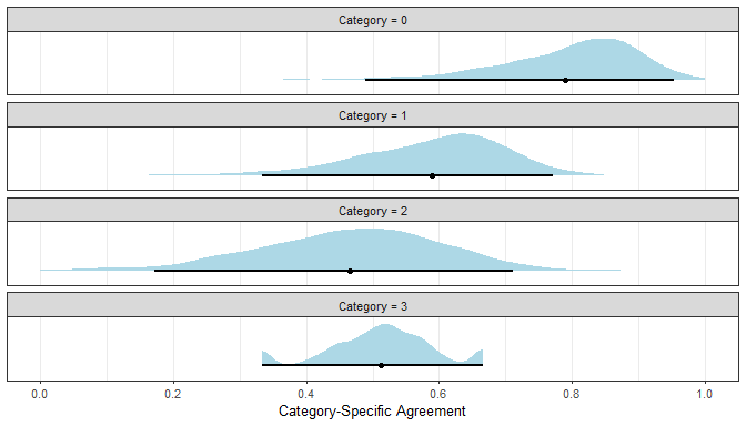
#>     Estimate   lower   upper
#> 0      0.812   0.461   0.948
#> 1      0.605   0.369   0.792
#> 2      0.483   0.242   0.767
#> 3 0.519 0.333 0.667tidy(results3, type = "bca")
#> # A tibble: 4 x 5
#> approach category estimate lower upper
#> <chr> <dbl> <dbl> <dbl> <dbl>
#> 1 Specific Agreement 0 0.812 0.461 0.948
#> 2 Specific Agreement 1 0.605 0.369 0.792
#> 3 Specific Agreement 2 0.483 0.242 0.767
#> 4 Specific Agreement 3 0.519 0.333 0.667plot(results3)Calculate intraclass correlation coefficient for dimensional data with 1 trial
# Load dataset with 4 raters rating 15 objects in 1 trial
data(lungfun)
print(lungfun)
#> # A tibble: 60 x 3
#>    Object Rater Score
#>     <int> <chr> <dbl>
#>  1      1 R1      190
#>  2      1 R2      220
#>  3      1 R3      200
#>  4      1 R4      200
#>  5      2 R1      220
#>  6      2 R2      200
#>  7      2 R3      240
#>  8      2 R4      230
#>  9      3 R1      260
#> 10      3 R2      260
#> # ... with 50 more rows
# Calculate average score ICC using Model 1A
results4 <- dim_icc(lungfun, model = "1A", type = "agreement", unit = "average",
object = Object, rater = Rater, score = Score, warnings = FALSE)
summary(results4)
#>
#> Intraclass Correlation Coefficient Analysis Details
#>
#> Number of Objects 15
#> Number of Raters 4
#> Number of Trials 1
#>
#> Score Missingness 0.000 %
#> Score Number Range [190, 375]
#>
#> ICC Model Model 1A
#> ICC Type Agreement
#> ICC Index Average of 4 Raters
#>
#> Variance Component Estimates with Bootstrapped CIs
#>
#> Estimate 2.5 % 97.5 %
#> Object Variance 1415.913 418.430 2477.863
#> Residual Variance 468.194 154.708 909.378
#>
#> ICC Estimates with Bootstrapped CIs
#>
#> Estimate 2.5 % 97.5 %
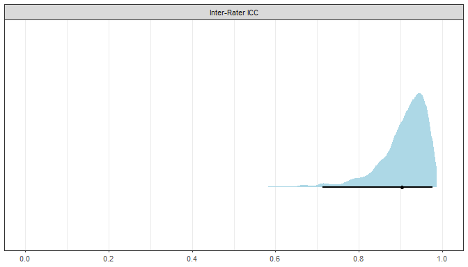
#> Inter-Rater ICC 0.924 0.713 0.977tidy(results4)
#> # A tibble: 3 x 4
#> term estimate lower upper
#> <chr> <dbl> <dbl> <dbl>
#> 1 Object Variance 1416. 418. 2478.
#> 2 Residual Variance 468. 155. 909.
#> 3 Inter-Rater ICC 0.924 0.713 0.977plot(results4, intra = FALSE, inter = TRUE)Calculate intraclass correlation coefficient for dimensional data with many trials
# Load dataset with 4 raters rating 8 objects in 3 trials
data(lungfun_trials)
print(lungfun_trials)
#> # A tibble: 59 x 4
#>    Object Rater Trial Score
#>     <dbl> <dbl> <dbl> <dbl>
#>  1      1     1     1   190
#>  2      1     1     2   220
#>  3      1     2     1   220
#>  4      1     2     2   200
#>  5      1     3     1   200
#>  6      1     3     2   240
#>  7      1     4     1   200
#>  8      1     4     2   230
#>  9      2     1     1   260
#> 10      2     1     2   210
#> # ... with 49 more rows
# Calculate single score ICC using Model 2A
results5 <- dim_icc(lungfun_trials, Object, Rater, Score, trial = Trial, model = "2",
type = "agreement", unit = "single", warnings = FALSE)
summary(results5)
#>
#> Intraclass Correlation Coefficient Analysis Details
#>
#> Number of Objects 8
#> Number of Raters 4
#> Number of Trials 3
#>
#> Score Missingness 41.667 %
#> Score Number Range [190, 375]
#>
#> ICC Model Model 2
#> ICC Type Agreement
#> ICC Index Single Rater
#>
#> Variance Component Estimates with Bootstrapped CIs
#>
#> Estimate 2.5 % 97.5 %
#> Object Variance 1652.014 299.866 3031.679
#> Rater Variance 97.109 3.254 347.156
#> Interaction (OxR) Variance -102.240 -375.003 -13.511
#> Residual Variance 461.333 217.335 807.058
#>
#> ICC Estimates with Bootstrapped CIs
#>
#> Estimate 2.5 % 97.5 %
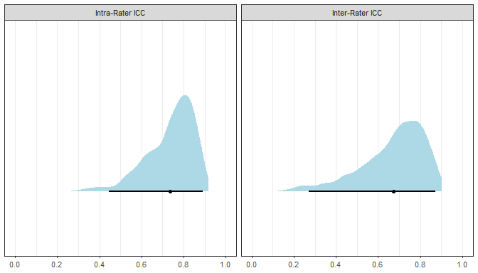
#> Intra-Rater ICC 0.791 0.446 0.892
#> Inter-Rater ICC 0.747 0.272 0.872tidy(results5)
#> # A tibble: 6 x 4
#> term estimate lower upper
#> <chr> <dbl> <dbl> <dbl>
#> 1 Object Variance 1652. 300. 3032.
#> 2 Rater Variance 97.1 3.25 347.
#> 3 O-by-R Variance -102. -375. -13.5
#> 4 Residual Variance 461. 217. 807.
#> 5 Intra-Rater ICC 0.791 0.446 0.892
#> 6 Inter-Rater ICC 0.747 0.272 0.872plot(results5)Please note that the ‘agreement’ project is released with a Contributor Code of Conduct. By contributing to this project, you agree to abide by its terms.

