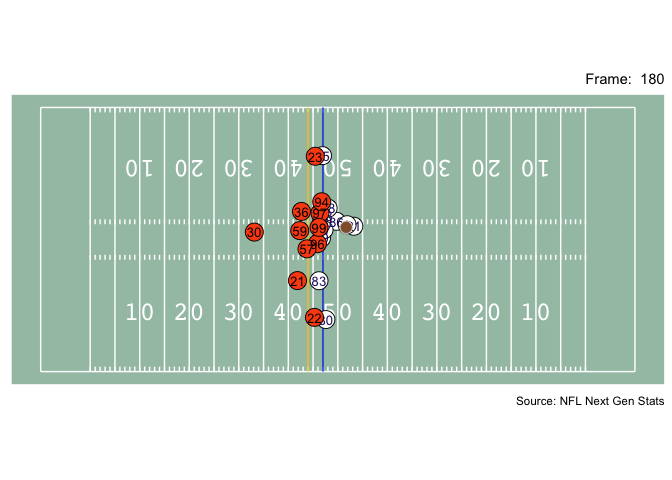
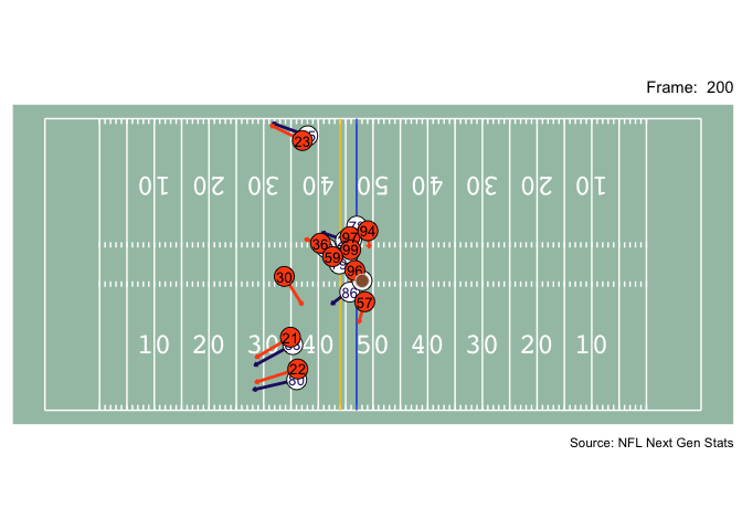
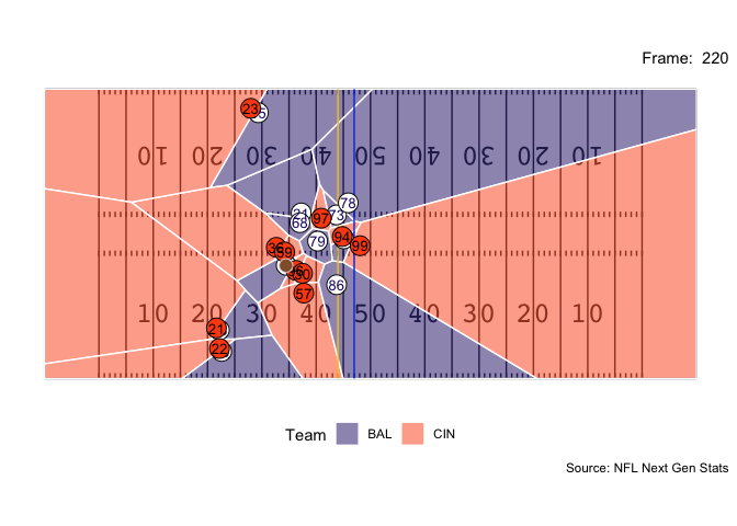
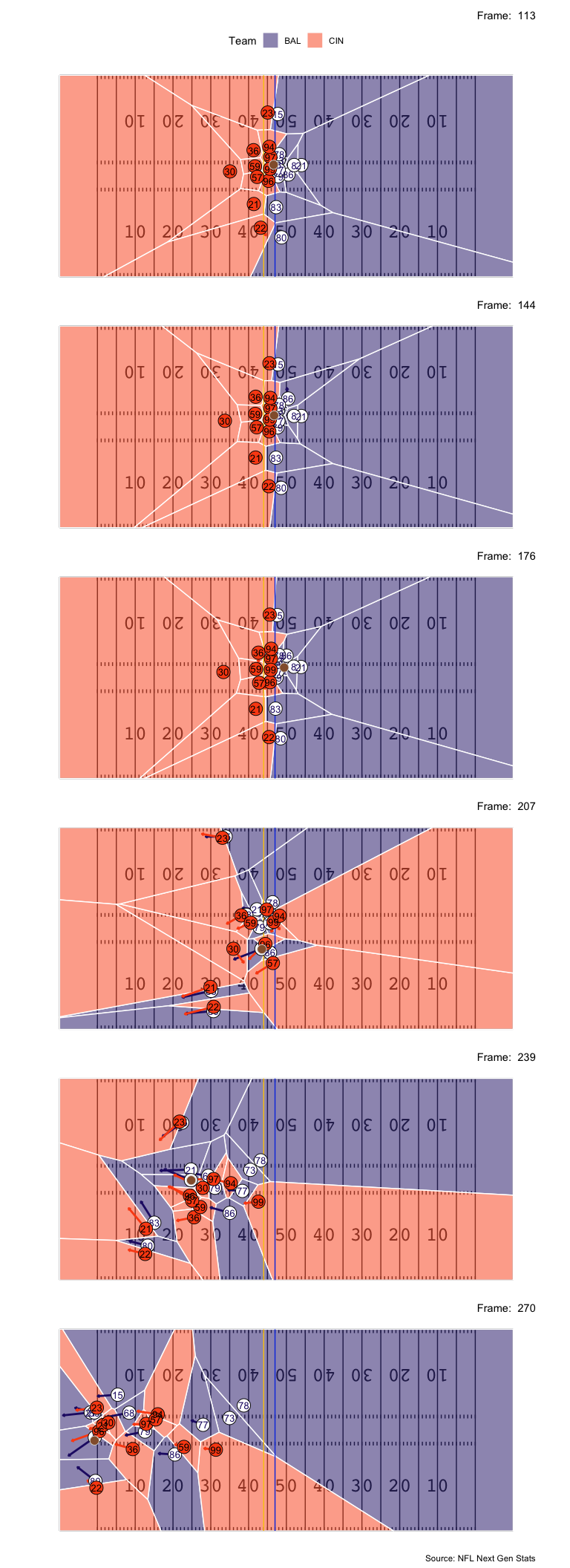
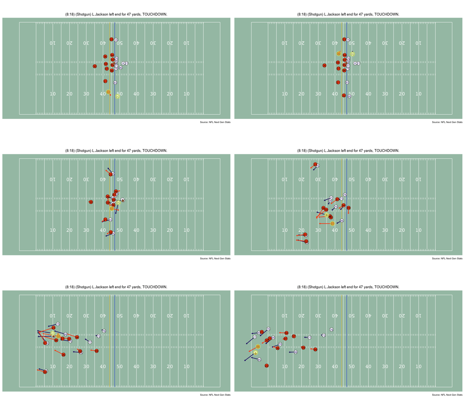
Getting Started With NFL Highlights Tracking Data

This is meant to be a very simple introduction to working with the tracking data housed in this repo. For a more in-depth guide on working with the NFL’s tracking data, check out Mike Lopez’s notebook from the most recent Big Data Bowl.

Intro

Tracking data has been billed as “the future of sports analytics,” but it’s notoriously difficult to both acquire and use. This repo was created to help alleviate those issues; it contains tracking data from the NFL’s Next Gen Stats (NGS) Highlights from the 2017-2019 seasons, as well as a few Rscripts with helper functions to make it easier to work with the data.

In this walk-through, we will:

import an NGS Highlight play’s tracking data
plot the frames from a play (with some extras)
animate a play

Setting Things Up

Before getting started with the data, we need to install and load a few libraries, as well as the Rscripts containing helper functions.

# * install packages ----
install.packages("devtools", "tidyverse")
devtools::install_github('thomasp85/ggforce')
devtools::install_github('thomasp85/gganimate')

# * load packages ----
library(devtools)
library(dplyr)
library(gganimate)
library(ggforce)
library(ggplot2)
library(readr)

# * load helper functions ----
source_url("https://raw.githubusercontent.com/asonty/ngs_highlights/master/utils/scripts/data_utils.R")
source_url("https://raw.githubusercontent.com/asonty/ngs_highlights/master/utils/scripts/plot_utils.R")

Importing the Data

Listing the Highlights

We can use the fetch_highlights_list() function to grab a list of the NGS Highlights in this repo, and by using the team_ and season_ arguments, we can filter the list down.

Lamar Jackson had some ridiculous plays during his MVP season, so let’s look at the Ravens’ highlights from 2019:

highlights <- fetch_highlights_list(team_ = "BAL", season_ = 2019)

playKey	playDesc	team	season	week	gameId	playId
237	(13:56) (Shotgun) L.Jackson pass deep middle to W.Snead for 33 yards, TOUCHDOWN.	BAL	2019	1	2019090803	1082
238	(4:28) (Shotgun) L.Jackson pass deep middle to M.Brown for 83 yards, TOUCHDOWN.	BAL	2019	1	2019090803	683
239	(8:12) (Shotgun) L.Jackson pass deep right to M.Andrews for 27 yards, TOUCHDOWN.	BAL	2019	2	2019091500	343
240	(1:24) (Shotgun) J.Hurst reported in as eligible. L.Jackson right tackle for 8 yards, TOUCHDOWN.	BAL	2019	7	2019102010	2997
241	(5:11) (Shotgun) R.Wilson pass short right intended for J.Brown INTERCEPTED by M.Peters at BLT 33. M.Peters for 67 yards, TOUCHDOWN.	BAL	2019	7	2019102010	1654
242	(8:18) (Shotgun) L.Jackson left end for 47 yards, TOUCHDOWN.	BAL	2019	10	2019111001	2257
243	(11:49) (Shotgun) L.Jackson right end to BLT 48 for 3 yards. Lateral to R.Griffin III pushed ob at CIN 43 for 9 yards (J.Bates III).	BAL	2019	10	2019111001	1000
244	(4:12) (Shotgun) G.Edwards left guard for 63 yards, TOUCHDOWN.	BAL	2019	11	2019111700	4243
245	(9:11) (Shotgun) L.Jackson left tackle to HST 20 for 39 yards (J.Reid). HST-L.Johnson was injured during the play.	BAL	2019	11	2019111700	2795
246	(9:54) (Shotgun) L.Jackson pass short middle to W.Snead IV for 4 yards, TOUCHDOWN. Caught at goal line, crossing to right.	BAL	2019	14	2019120801	3526
247	(13:44) (Shotgun) L.Jackson pass deep left to H.Hurst for 61 yards, TOUCHDOWN [J.Hughes]. Flag pattern, caught at BUF 41.	BAL	2019	14	2019120801	2271
248	(1:04) (Shotgun) L.Jackson pass deep left to S.Roberts for 33 yards, TOUCHDOWN. Lamar Jackson’s 4th TD pass of game and 32nd of season.	BAL	2019	15	2019121200	2839
249	(5:14) (Shotgun) L.Jackson pass deep middle to M.Brown for 24 yards, TOUCHDOWN.	BAL	2019	15	2019121200	2486
250	(13:40) (Shotgun) L.Jackson right guard pushed ob at TEN 42 for 27 yards (W.Woodyard).	BAL	2019	19	2020011101	3181
251	(12:16) (Shotgun) L.Jackson scrambles left guard to TEN 27 for 30 yards (L.Ryan).	BAL	2019	19	2020011101	2230
252	(:18) (Shotgun) L.Jackson pass deep right to M.Brown to TEN 04 for 38 yards (A.Hooker).	BAL	2019	19	2020011101	1899

Importing the Tracking Data

The first column in the table (playKey) is a unique identifier for each play in the dataset, and is used by the fetch_play_data() function to grab the tracking data for a play. Let’s take a look at Lamar Jackson’s 47-yard touchdown run. The playKey for that play is 242, so we’ll provide that to fetch_play_data().

play_data <- fetch_play_data(playKey_ = 242)

gameId	playId	playType	season	seasonType	week	preSnapHomeScore	preSnapVisitorScore	playDirection	quarter	gameClock	down	yardsToGo	yardline	yardlineSide	yardlineNumber	absoluteYardlineNumber	homeTeamFlag	teamAbbr	frame	displayName	esbId	gsisId	jerseyNumber	nflId	position	positionGroup	time	x	y	s	o	dir	event	playDescription
2019111001	2257	play_type_rush	2019	REG	10	10	28	left	3	08:18:00	2	3	CIN 47	CIN	47	57	1	CIN	0	Geno Atkins	ATK216644	00-0027720	97	496762	DT	DL	2019-11-10 19:46:19	54.74	29.83	0.01	80.80	95.59	huddle_start_offense	(8:18) (Shotgun) L.Jackson left end for 47 yards, TOUCHDOWN.
2019111001	2257	play_type_rush	2019	REG	10	10	28	left	3	08:18:00	2	3	CIN 47	CIN	47	57	1	CIN	1	Geno Atkins	ATK216644	00-0027720	97	496762	DT	DL	2019-11-10 19:46:19	54.74	29.83	0.01	80.80	98.23	NA	(8:18) (Shotgun) L.Jackson left end for 47 yards, TOUCHDOWN.
2019111001	2257	play_type_rush	2019	REG	10	10	28	left	3	08:18:00	2	3	CIN 47	CIN	47	57	1	CIN	2	Geno Atkins	ATK216644	00-0027720	97	496762	DT	DL	2019-11-10 19:46:20	54.74	29.83	0.01	81.44	94.54	NA	(8:18) (Shotgun) L.Jackson left end for 47 yards, TOUCHDOWN.
2019111001	2257	play_type_rush	2019	REG	10	10	28	left	3	08:18:00	2	3	CIN 47	CIN	47	57	1	CIN	3	Geno Atkins	ATK216644	00-0027720	97	496762	DT	DL	2019-11-10 19:46:20	54.74	29.84	0.01	81.44	86.27	NA	(8:18) (Shotgun) L.Jackson left end for 47 yards, TOUCHDOWN.
2019111001	2257	play_type_rush	2019	REG	10	10	28	left	3	08:18:00	2	3	CIN 47	CIN	47	57	1	CIN	4	Geno Atkins	ATK216644	00-0027720	97	496762	DT	DL	2019-11-10 19:46:20	54.74	29.84	0.01	81.44	84.09	NA	(8:18) (Shotgun) L.Jackson left end for 47 yards, TOUCHDOWN.

Visualizing Plays

In my opinion, the most fun way to get started with tracking data is through visualizations. To that end, we can use the plot_play_frame() function to plot any given frame in a play.

It’s important to note that the tracking data contains the entire runtime of the play, including all of the dead time prior to the line being set, and in some cases even the team celebrations after a touchdown is scored. So let’s first find the ‘frame interval’ of the play:

first_frame <- play_data %>%
  filter(event == "line_set") %>% 
  distinct(frame) %>% 
  slice_max(frame) %>% 
  pull()

final_frame <- play_data %>% 
  filter(event == "tackle" | event == "touchdown" | event == "out_of_bounds") %>% 
  distinct(frame) %>% 
  slice_max(frame) %>% 
  pull()

first_frame

## [1] 113

final_frame

## [1] 270

Basic Play Frame Plot

Now that we’ve got a better idea of the interval in which the play takes place, let’s visualize it.

plot_play_frame(play_data_ = play_data, frame_ = 180)

Play Frame Plot + Velocity Vectors

plot_play_frame() also has a velocities_ parameter, which, when set to TRUE, adds the players’ velocity vectors to the plot.

plot_play_frame(play_data_ = play_data, frame_ = 200, velocities_ = T)

Play Frame Plot + Voronoi Tessellation

In past Big Data Bowls, some of the top submissions borrowed a concept from soccer called “pitch control.” Pitch control models aim to quantify the areas of the field that players/teams control; an example of a basic pitch control model is Voronoi tessellation. We can use the voronoi_ argument to add a Voronoi layer to play frame plots:

plot_play_frame(play_data_ = play_data, frame_ = 220, velocities_ = F, voronoi_ = T)

The final in-built function we can use is plot_play_sequence(), which plots n_ number of frames between a first_frame_ and final_frame_ at evenly spaced intervals:

plot_play_sequence(play_data, first_frame_ = first_frame, final_frame_ = final_frame, n_ = 6, velocities_ = T, voronoi_ = T)

Animating a Play

The next step in visualizing a play is animation. Rather than just animating the data as-is, let’s transform it a bit. In our animation, we’re going to highlight the fastest player on each team at every frame of the play.

Data Manipulation

First, we’ll reduce the dataset, split it up into player and ball data, and grab some details.

# * reduce dataset ----
reduced_play_data <- play_data %>% filter(frame >= first_frame, frame <= final_frame+10)

# * get play details ----
play_desc <- reduced_play_data$playDescription %>% .[1]
play_dir <- reduced_play_data$playDirection %>% .[1]
yards_togo <- reduced_play_data$yardsToGo %>% .[1]
los <- reduced_play_data$absoluteYardlineNumber %>% .[1]
togo_line <- if(play_dir=="left") los-yards_togo else los+yards_togo

# * separate player and ball tracking data ----
player_data <- reduced_play_data %>% 
  select(frame, homeTeamFlag, teamAbbr, displayName, gsisId, jerseyNumber, position, positionGroup,
         x, y, s, o, dir, event) %>% 
  filter(displayName != "ball")
ball_data <- reduced_play_data %>% 
  select(frame, homeTeamFlag, teamAbbr, displayName, jerseyNumber, position, positionGroup,
         x, y, s, o, dir, event) %>% 
  filter(displayName == "ball")

# * get team details ----
h_team <- reduced_play_data %>% filter(homeTeamFlag == 1) %>% distinct(teamAbbr) %>% pull()
a_team <- reduced_play_data %>% filter(homeTeamFlag == 0) %>% distinct(teamAbbr) %>% pull()
#  call helper function to get team colors
team_colors <- fetch_team_colors(h_team_ = h_team, a_team_ = a_team)
h_team_color1 <- team_colors[1]
h_team_color2 <- team_colors[2]
a_team_color1 <- team_colors[3]
a_team_color2 <- team_colors[4]

Next, we’ll compute the x and y component’s of each player’s velocity. Note that the dir variable specifies the direction of the player’s movement; it is 0 degrees when the player is facing ‘up’ on the field (towards the far sideline) and increases in the clockwise direction.

# * compute velocity components ----
#  velocity angle in radians
player_data$dir_rad <- player_data$dir * pi / 180

#  velocity components
player_data$v_x <- sin(player_data$dir_rad) * player_data$s
player_data$v_y <- cos(player_data$dir_rad) * player_data$s

Finally, we’ll identify the fastest players on each team in every frame, and merge that information with our player_data:

#  there are assuredly better ways to do this

# * identify the fastest player from each team at each frame ----
fastest_players <- player_data %>% # filter out ball-tracking data
  group_by(frame, teamAbbr) %>% # group by frame and team
  arrange(s) %>% top_n(s, n=1) %>% # take only the players with the highest speed on each team at every frame
  mutate(isFastestFlag = 1) %>% # create new flag identifying fastest players
  ungroup() %>% 
  select(frame, gsisId, isFastestFlag) %>%  # reduce dataset to the columns needed for joining and the new flag
  arrange(frame) # sort by frame

player_data <- player_data %>% 
  left_join(fastest_players, by = c("frame" = "frame", "gsisId" = "gsisId")) %>% # join on frame and gsisId
  mutate(isFastestFlag = case_when(is.na(isFastestFlag) ~ 0, TRUE ~ 1)) # replace NA values for isFastestFlag with 0

Animating the Play

Unfortunately, we can’t just use the plot_play_frame() function to animate a play, so we’re going to peel back the function’s innards to create our animation.

play_frames <- plot_field() + # plot_field() is a helper function that returns a ggplot2 object of an NFL field
  # line of scrimmage
  annotate(
    "segment",
    x = los, xend = los, y = 0, yend = 160/3,
    colour = "#0d41e1"
  ) +
  # 1st down marker
  annotate(
    "segment",
    x = togo_line, xend = togo_line, y = 0, yend = 160/3,
    colour = "#f9c80e"
  ) +
  # away team velocities
  geom_segment(
    data = player_data %>% filter(teamAbbr == a_team),
    mapping = aes(x = x, y = y, xend = x + v_x, yend = y + v_y),
    colour = a_team_color1, size = 1, arrow = arrow(length = unit(0.01, "npc"))
  ) + 
  # home team velocities
  geom_segment(
    data = player_data %>% filter(teamAbbr == h_team),
    mapping = aes(x = x, y = y, xend = x + v_x, yend = y + v_y),
    colour = h_team_color1, size = 1, arrow = arrow(length = unit(0.01, "npc"))
  ) +
  # away team locations
  geom_point(
    data = player_data %>% filter(teamAbbr == a_team),
    mapping = aes(x = x, y = y),
    fill = "#ffffff", color = a_team_color2,
    shape = 21, alpha = 1, size = 6
  ) +
  # away team jersey numbers
  geom_text(
    data = player_data %>% filter(teamAbbr == a_team),
    mapping = aes(x = x, y = y, label = jerseyNumber),
    color = a_team_color1, size = 3.5, #family = "mono"
  ) +
  # home team locations
  geom_point(
    data = player_data %>% filter(teamAbbr == h_team),
    mapping = aes(x = x, y = y),
    fill = h_team_color1, color = h_team_color2,
    shape = 21, alpha = 1, size = 6
  ) +
  # home team jersey numbers
  geom_text(
    data = player_data %>% filter(teamAbbr == h_team),
    mapping = aes(x = x, y = y, label = jerseyNumber),
    color = h_team_color2, size = 3.5, #family = "mono"
  ) +
  # ball location
  geom_point(
    data = ball_data,
    mapping = aes(x = x, y = y),
    fill = "#935e38", color = "#d9d9d9",
    shape = 21, alpha = 1, size = 4
  ) +
  # highlight fastest players
  geom_point(
    data = player_data %>% filter(isFastestFlag == 1),
    mapping = aes(x = x, y = y),
    colour = "#e9ff70",
    alpha = 0.5, size = 8
  ) +
  # play description and always cite your data source!
  labs(
    title = play_desc,
    caption = "Source: NFL Next Gen Stats"
  ) + 
  # animation stuff
  transition_time(frame) +
  ease_aes('linear') +
  NULL

# ensure timing of play matches 10 frames-per-second (h/t NFL Football Ops)
play_length <- length(unique(player_data$frame))
play_anim <- animate(
  play_frames,
  fps = 10, 
  nframe = play_length,
  width = 850,
  height = 500,
  end_pause = 10
)

asonty / ngs_highlights