BEGAN: Boundary Equibilibrium Generative Adversarial Networks

This is an implementation of the paper on Boundary Equilibrium Generative Adversarial Networks (Berthelot, Schumm and Metz, 2017).

Dependencies

Python 3+
numpy
Tensorflow
tqdm
h5py
scipy (optional)

What are Boundary Equilibrium Generative Adversarial Networks?

Unlike standard generative adversarial networks (Goodfellow et al. 2014), boundary equilibrium generative adversarial networks (BEGAN) use an auto-encoder as a disciminator. An auto-encoder loss is defined, and an approximation of the Wasserstein distance is then computed between the pixelwise auto-encoder loss distributions of real and generated samples.

With the auto-encoder loss defined (above), the Wasserstein distance approximation simplifies to a loss function wherein the discriminating auto-encoder aims to perform well on real samples and poorly on generated samples, while the generator aims to produce adversarial samples which the discriminator can't help but perform well upon.

Additionally, a hyper-parameter gamma is introduced which gives the user the power to control sample diversity by balancing the discriminator and generator.

Gamma is put into effect through the use of a weighting parameter k which gets updated while training to adapt the loss function so that our output matches the desired diversity. The overall objective for the network is then:

Unlike most generative adversarial network architectures, where we need to update G and D independently, the Boundary Equilibrium GAN has the nice property that we can define a global loss and train the network as a whole (though we still have to make sure to update parameters with respect to the relative loss functions)

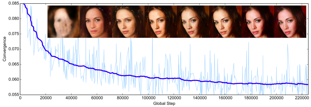
The final contribution of the paper is a derived convergence measure M which gives a good indicator as to how the network is doing. We use this parameter to track performance, as well as control learning rate.

The overall result is a surprisingly effective model which produces samples well beyond the previous state of the art.

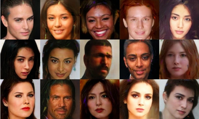
128x128 samples generated from random points in Z, from (Berthelot, Schumm and Metz, 2017).

Usage

Data Preprocessing

You might want to use the 'CelebA' dataset (Liu et al. 2015), this can be downloaded from the project website. Make sure to download the 'Aligned and Cropped' Version. However you can modify these instructions to use an alternate dataset.

(Note: if the CelebA Dropbox is down you can alternatively use their Google Drive).

This then needs to be prepared into hdf5 through the following method:

from glob import glob 
import os
import numpy as np
import h5py
from tqdm import tqdm
from scipy.misc import imread, imresize

filenames = glob(os.path.join("img_align_celeba", "*.jpg"))
filenames = np.sort(filenames)
w, h = 64, 64  # Change this if you wish to use larger images
data = np.zeros((len(filenames), w * h * 3), dtype = np.uint8)

# This preprocessing is appriate for CelebA but should be adapted
# (or removed entirely) for other datasets.

def get_image(image_path, w=64, h=64):
    im = imread(image_path).astype(np.float)
    orig_h, orig_w = im.shape[:2]
    new_h = int(orig_h * w / orig_w)
    im = imresize(im, (new_h, w))
    margin = int(round((new_h - h)/2))
    return im[margin:margin+h]

for n, fname in tqdm(enumerate(filenames)):
    image = get_image(fname, w, h)
    data[n] = image.flatten()

with h5py.File(''.join(['datasets/celeba.h5']), 'w') as f:
    f.create_dataset("images", data=data)

Training

After your dataset has been created through the method above, change the file config.py to point to your dataset, and to point to your desired checkpoint directory.

E.g., if your dataset is stored at /home/user/data/dataset.hdf5, then alter config.py to read:

dataset_path = '/home/user/data/dataset.hdf5'
checkpoint_path = './checkpoints'

You can then begin training:

python main.py --start-epoch=0, add-epochs=100 --save-every 5

If you have limited RAM you might need to limit the number of images loaded into memory at once, e.g.

python main.py --start-epoch=0 add-epochs=100 --save-every 5 --max-images 20000

I have 12GB which works for around 60,000 images.

You can specify GPU id with the --gpuid argument. If you want to run on CPU (not recommended!) use --gpuid -1

Other parameters can be tuned if you wish (run python main.py --help for the full list). The default values are the same as in the paper (though the authors point out that their choices aren't necessarily optimal).

The main difference between this implementation's defaults and the original paper is the use of batch normalisation, we found that not using batch normalisation made training much slower.

Running

After you've trained a model and you want to generate some samples simply run

python main.py --start-epoch=N add-epochs=0 --train=False

where N is the checkpoint you want to run from. Samples will be saved to ./outputs/ by default (or add optional argument --outdir for alternative).

Tracking Progress

As discussed previously, the convergence measure gives a very nice way of tracking progress This is implemented into the code (via the dictionary loss_tracker with key convergence_measure)

Berthelot, Schumm and Metz show that it is a true-to-reality metric to use:

Convergence measure over training epochs, with generator outputs showed above (Berthelot, Schumm and Metz, 2017).

Issues / Contributing / Todo

Feel free to raise any issues in the project issue tracker, or make a pull-request if there is something you want to add.

My next plan is to upload some pre-trained weights so beginners can run the model out-of-the-box.

artcg / BEGAN