-
Arnald Marcer
- CREAF, Cerdanyola del Vallès 08193, Spain
- Univ. Autòonoma de Barcelona, Cerdanyola del Vallès, Spain -
F. Xavier Picó
- Departamento de Ecología Integrativa, Estación Biológica de Doñana (EBD), Consejo Superior de Investigaciones Científicas (CSIC), Sevilla 41092, Spain
- Background
- Historical orthoimages dataset
- HistHab applications
- Configuration and server-side
- References
Preliminary note: The following applications have been developed with the aim of building a historial database of land cover around wild populations of Arabidopsis thaliana in the Iberian peninsula, and what is here explained is tailored to that end. However, the tool can be accomodated to other species and study areas with a small development effort.
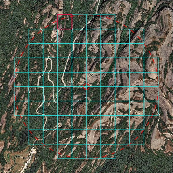
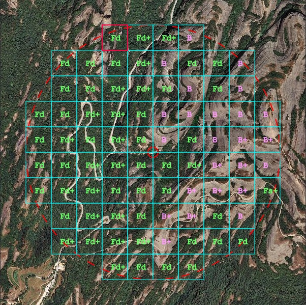
This application is designed to make historical local maps of land cover around natural populations of Arabidopsis thaliana. These maps are circular buffers of a given radius (500 meters) around a central population coordinate and are discretized in square units of a given size (100 meters) (Figure 1) which can be manually labelled with a given land cover category (Figure 2). The category is assigned according to the criterion of predominant land cover category in the square (largest area). Currently, land cover categories are fixed within the application (see below). For each population there are as many orthoimages as years available.
Figure 1. Land cover data grid over 2013 orthoimage for population *El Brull* . Grid squares are included if their central point is inside the circular buffer (in red). Figure 2. Already filled land cover data grid.For the Historical land cover and Data validation applications to be used, historical orthophotographies need to be prepared beforehand. In the case of the Iberian peninsula, these have been obtained through the spatial data infrastructures of the central and regional governments with a python application (please refer to project https://github.com/arnaldmarcer/ath_hist).
The following applications are bundled together in a web page and together they allow to handle the photointerpretation and labelling of historical orthoimages.
This is a simple web page with a menu option, Open application, from which the rest of the applications can be accessed.
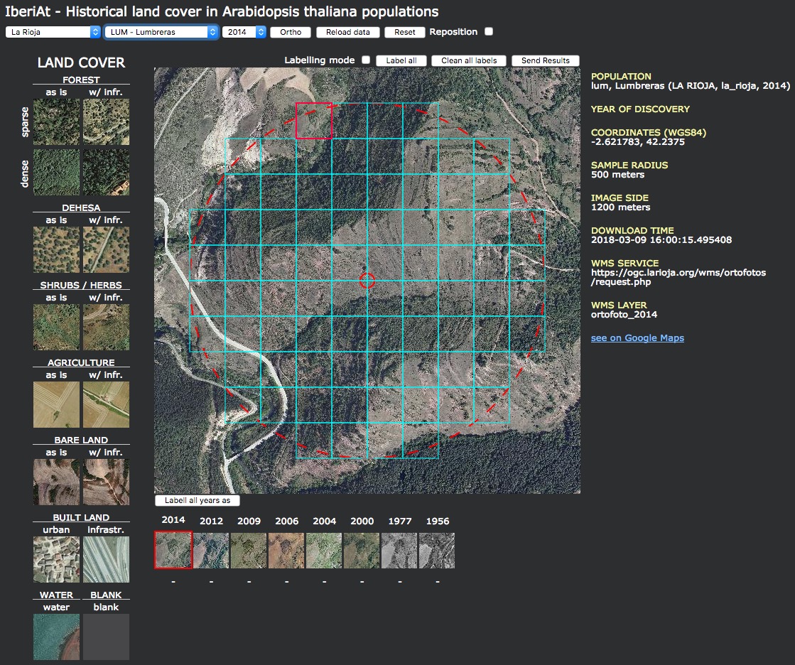
Figure 3. Web portal page. Applications are accessible in the menu 'Open application'.This is the main application (see Figure 4) which allows to label historical land cover categories (see Figure 1 and 2) for each orthoimage prepared (see [Historical orthoimages dataset] section above). Land cover categories have been preestablished and thougth in the context of natural environments in the Iberian peninsula. In order to use other categories some code tweaking would be necessary. As of this version the land cover categories are shown in the table below. Categories with a + sign mean that within the labelled square there is the presence of some sort of human element, e.g. road, building, etc.
| Land Cover | Label |
|---|---|
| Dense forest | Fd / Fd+ |
| Sparse forest | Fs / Fs+ |
| Dehesa | D / D+ |
| Shrubs / Herbs | S / S+ |
| Bare land | B / B+ |
| Urban | U |
| Infrastructures | I |
| Water | W |
As noted above, categories are assigned to each square in the grid according to a predominance criterion, i.e. the square is labelled with the land cover category with the largest area within it.
Figure 4. Graphical user interface for the data entry application.USAGE
- Use dropdown controls above page to select the population
- Ortho button: Shows only orthoimage
- Reload data button: Reloads data from server for the given population
- Reset button: Erases all labels and repositions population to original coordinates
- Reposition checkbox: Allows to relocate the population coordinates
- Labelling
- Check the Labelling mode checkbox.
- Select category in left-hand legend by clicking on corresponding image.
- Click on a given square in the grid to label it, to change the label simply select another category and click again.
- You may use the blank category to erase a single label in a given square grid.
- Label all button: Labels all grid squares with the selected category.
- Clean all labels button: Erases all labels from the grid of squares.
- Send results button: Saves results to server.
- IMPORTANT: Data is not saved automatically, the user needs to send results to server. Do so from time to time to avoid losing data.
- Timeline
- Below the main image there is a row of small images each of which correponds to the image for the different available historical orthoimages for the selected square in the main image.
- Labell all years as : Labels all images in the timeline row with the selected land cover category.
- Clicking on a given image in the timeline will load the corresponding historical orthoimage in the main image panel.
Image metadata
Metadata for the image is shown right to it.
- Population: Code, name, region of the population and year of the shown image.
- Year of discovery: Year in which the population was discovered.
- Coordinates (WGS84): Population coordinates in WGS84.
- Sample radius: Radius size of the big red sampling circle in the image.
- Image side: Size in meters of the shown image.
- Download time: When was the image downloaded from the corresponding spatial data infrastructure.
- WMS Service: URL of the cooresponding WMS service from which the image has been obtained.
- WMS Layer: Name of the WMS layer.
- see on Google Maps link: Opens a new window with the population shown in Google Maps.
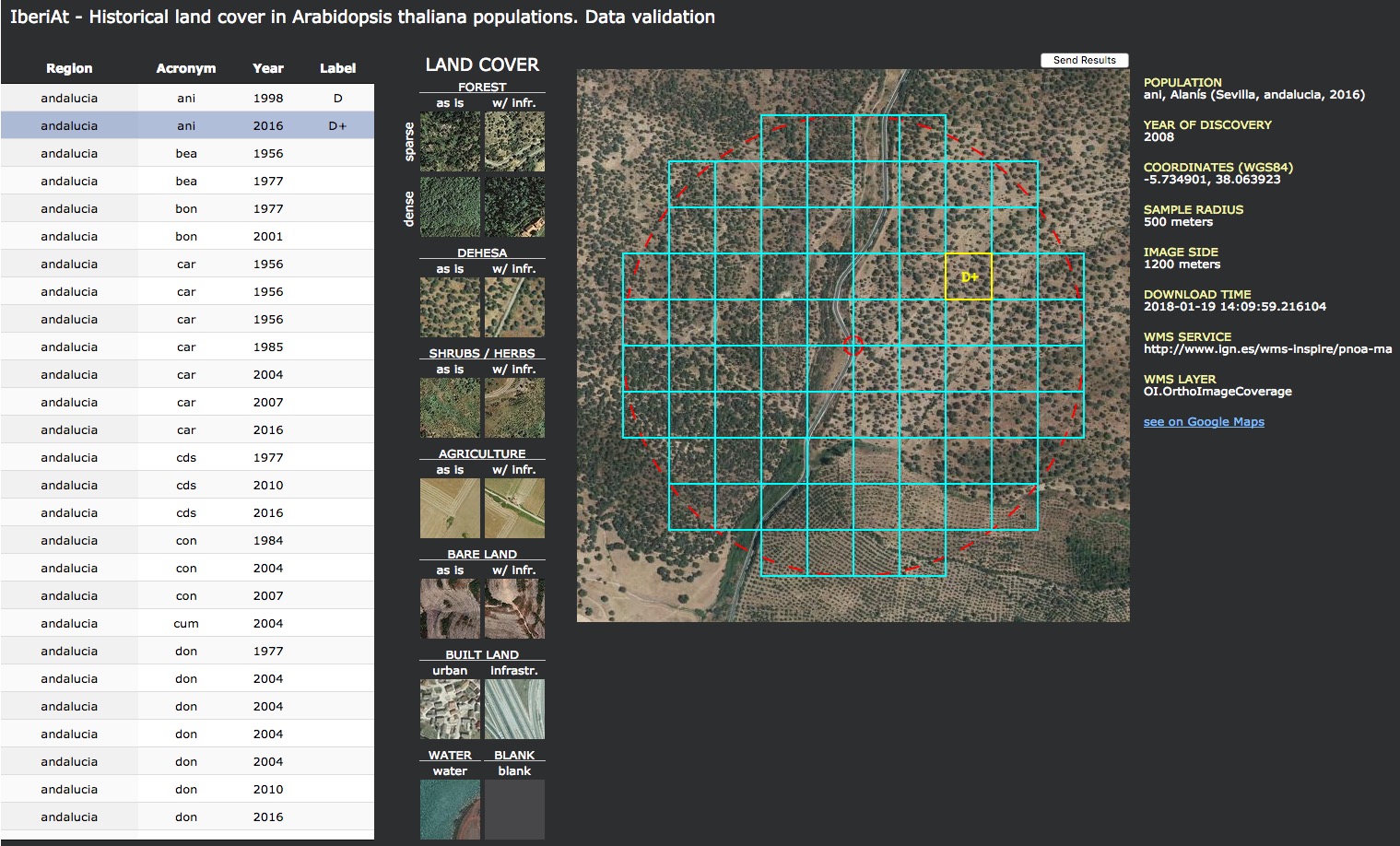
This is a complementary application to the Historical land cover data entry application (see above). Its purpose is to validate the data entered by a given photointerpreter. The application needs to be given a random list of squares among all populations and years in order to do the validation. A different photointerpreter than the one who performed the data entry process independently assigns land cover categories to the this selected random list of squares. If there is a high agreement between different photointerpreters which have labelled data independently then one can conclude that assigned land cover categories are robust.
Figure 5. Graphical user interface for the data validation application.USAGE
The table on the left contains the random squares validation dataset (see below).
- Click on a row in the table to select the square, the application will show the corresponding square highlighted over the square grid over the corresponding orthoimage.
- Click on the land cover category image in the legend to assign it to the square.
- Use the Send results button to save results to the server. This is not done automatically and the user needs to do it from time to time in order not to lose entered data.
The metadata on the right are the same as in the data entry application above.
Data are stored in a json file (see Configuration and setup section below).
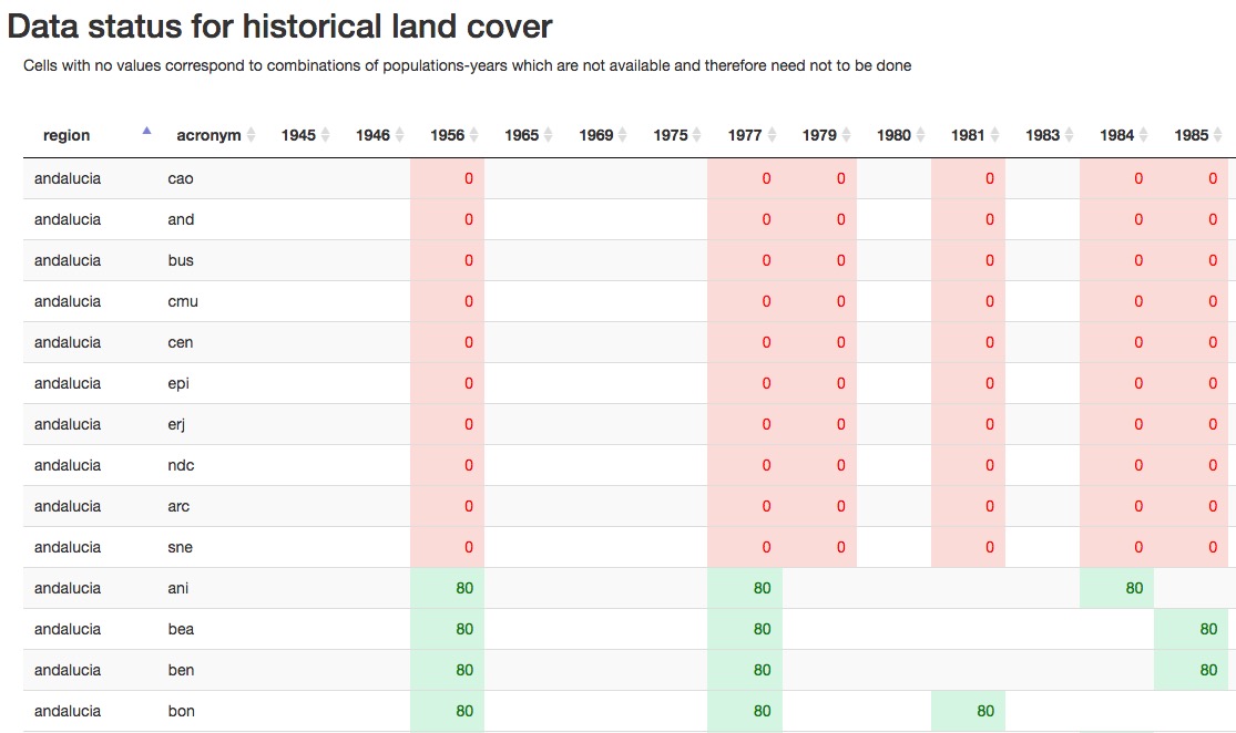
Figure 6. Data status applicaiton main windowThis a helping application for the person photointerpreter of the historical land cover. It shows a table with the status of each population data. A number is given for each population and year which represents the number of labelled squares. In this implementation, each population/year has 80 squares to be labelled and when this is complete is shown in green and when it is not, in red.
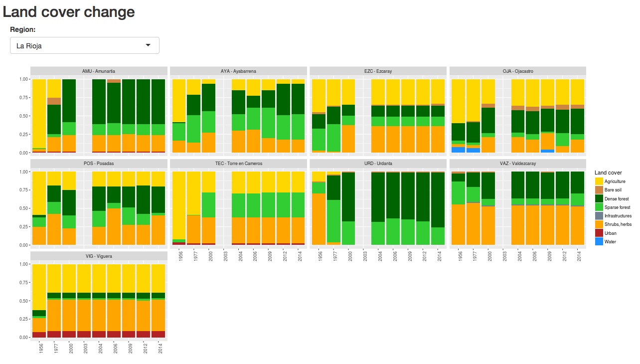
Figure 7. Land cover change per population.This is an application to make a simple representation of the data entered in the data entry application (see above). It outputs stacked bar plots which show the relative percentages of land cover per population and year. This application can also help the photointerpreter and validator to check for rare patterns in the data which may be further checked for errors in the interpretation process.
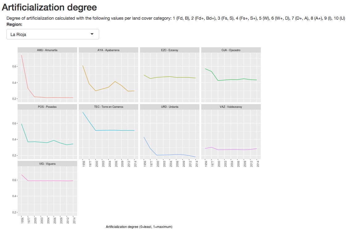
Figure 8. Degree of artificializationThis application calculates a simple index of artificialization and plots a line graph per population. It uses the data entered in the data entry application (see above). It outputs line graphs of the calculated articialization index against year for each population. This application can also help the photointerpreter and validator to check for rare patterns in the data which may be further checked for errors in the interpretation process.
In order to calculate the index a weight value is given to each land cover category:
1 (Fd, B), 2 (Fd+, Bd+), 3 (Fs, S), 4 (Fs+, S+), 5 (W), 6 (W+, D), 7 (D+, A), 8 (A+), 9 (I), 10 (U)
(see above for labels description)
This application is composed of the following files located in the html/ folder of this repository:
- home.html: Layout of the page
- home.css: Page style
- home.js: Javascript application code
- Dependencies:
- jquery-3.2.1.min.js: JQuery Javascript library
A directory named env/ located at the root of the repository must be present with the following configuration files:
apps.json
This file contains the references and URLs of the applications mentioned above. Its format must be as shown below with the <ip-number> and <port-number> set accordingly.
[{
    "application":"pophist",
    "name":"Data entry",
    "url": "http://<ip-number>:<port-number>/pophist/html/pophist.html"
},
{
    "application":"pophist_validation",
    "name":"Data validation",
    "url": "http://<ip-number>:<port-number>/pophist/html/pophist_validation.html"
},
{
    "application":"pophist_data_status",
    "name":"Data status",
    "url": "http://<ip-number>:<port-number>/pophist/shiny/data_status/"
},
{
    "application":"pophist_land_cover_change",
    "name":"Land cover change",
    "url": "http://<ip-number>:<port-number>/pophist/shiny/land_cover_change/"
},
{
    "application":"pophist_human_impact_degree",
    "name":"Human impact",
    "url": "http://<ip-number>:<port-number>/pophist/shiny/human_impact/"
}]
config.json
This files contains the folder location of the directory where the orthoimages and entered data are stored. Paths must be relative to the location of the js files, i.e. the html folder.
{
  "dir_results" : "<relative-path>",
  "dir_orthos" : "<relative-path>"
}
users.json
File containing the users and passwords. Format:
{
  "<user_name_1>":"<password_1>",
  "<user_name_2>":"<password_2>",
  "<user_name_3>":"<password_3>",
  ...
  "<user_name_N>":"<password_N>"
}
Orthoimages folder structure
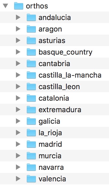
Orthoimages are stored in directory defined in the config.json file described above. This directory is accessible to the server application and within directories corresponding to the region in the Iberian peninsula where their corresponding population is located as in Figure 9 below.
Figure 9. Orthoimages folder structure.Orthoimages files and naming convention
Each orthoimage is represented by a jpg file and a json file, with the following naming pattern:
- ani_ortho_2010_r50_2km[.jpg/.json] (an example from the andalucia folder)
- Only the following substrings are variable:
- ani (code for the corresponding population)
- 2010 (year of the orthoimage)
- 50 (resolution in meters)
- Only the following substrings are variable:
The json file is automatically generated when downloading the orthoimage (see [Historical orthoimages dataset] section).
Entered data folder structure
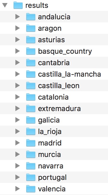
Entered data are stored in json files in a folder structure equal to the orthoimages folder structure but in a different root directory (as defined in the config.json file described above) as in Figure 10 below. A json for each population is saved and named after the population code or acronym. Data for all years are stored in this file. Squares' ids are numbered from 1 to n for all years altogether.
Figure 10. Results folder structure.Example of a results json file
This file would be named after the acronym of the population, that is ani.json.
{
  "acronym": "ani",
  "region": "andalucia",
  "xc": 500,
  "yc": 500
  "grid": [{
            "id": 1,
            "xc": 400,
            "yc": 250,
            "xs": 50,
            "ys": 50,
            "year": "2016",
            "label": "D",
            "user": "john",
            "timestamp": "01/01/2018, 12:36:58",
            "ip": "255.255.255.255"
          },
          {
            ...
          }]
}
Please note that as of this version of the application, downloaded images are 2000 meters by side and 2 meters resolution and centered on the population which they represent, hence the value of 500 for xc and yc.
Keys in the json file:
- acronym: Population code
- region: Region where the population is located
- xc: Population x coordinate in image pixels
- yc: Population y coordinate in image pixels
- grid: List of squares in which the labelling is divided
- id: Square id or number within the square grid (see Figure 1)
- xc: Minimum x in image pixels for the given square
- yc: Maximum y in image pixels for the given square
- xs: Square x size in pixels
- ys: Square y size in pixels
- year: Orthoimage year
- label: Assigned land cover category
- user: User name of the person who labelled the square
- timestamp: Timestamp for when the square was labelled
- ip: IP of the computer from which the square was labelled
Aplication files
This application is composed of the following files located in the html/ directory of this repository:
- pophist.html: Layout of the page
- pophist.css: Page style
- pophist.js: Javascript application code
- Dependencies:
- jquery-3.2.1.min.js: JQuery Javascript library
- underscore-min.js: Underscore Javascript library
The application uses the same orthoimages from the same folder structure as the Historical land cover application above. The only extra data needed is the validation dataset, which is explained below. This is a dataset stored as a json file named as <user_check>_accuracy_assessment_sample.json in the same folder as the results of the Historical land cover application (see above). <user_check> is the name of the user doing the validation. This allows for doing different validations by different persons. Validation data entered with this application are stored in this same json file.
Validation json file
The number of random grid squares for the validating sample can be calculated according to Congalton & Green (2008)(pp. 74 -- 79) with the following R function:
getClassSampleSize <- function(){
  p <- 0.5 # Estimated percentage for category closest to 0.5
           # We use 0.5 to be conservative
  alpha <- 0.05
  k <- length(labels)
  chisq.value <- qchisq(1 - alpha/k,1)
  overall.sample.size <- ceiling(chisq.value * p * (1 - p) / alpha^2)
  cat("\nOverall sample size: ", overall.sample.size)
  sample.size.per.class <- ceiling(overall.sample.size / k)
  cat("\nPer class sample size: ", sample.size.per.class)
  return(sample.size.per.class)
}
An overall number of needed squares is computed and then divided by the number of land cover categories. Then we can sample the overall dataset of squares for all populations and years and extract this number of random squares per category with the following R command:
df.s <- df %>% na.omit() %>% group_by(label) %>% sample_n(class.sample.size)
where df is a dataframe containing all squares accross all populations and years, label is the dataframe column containing the land cover category and class.sample.size is the sample size per class as calculated with the above R function.
Once the df.s dataframe containing the validation dataset is obtained, it is saved as the json file mentioned above. Its format is:
[{
  "acronym": "ace",
  "region": "extremadura",
  "resolution": 50,
  "year": 1980,
  "pop_xc": 500,
  "pop_yc": 500,
  "xc": 350,
  "yc": 300,
  "xs": 50,
  "ys": 50,
  "id_json": 646,
  "id": 6,
  "user": "john",
  "label": "D",
  "user_check": "",
  "label_check": "",
  "timestamp_check": "",
 },
 {
  ...
 }]
Keys in the json file:
- acronym: Population code
- region: Region where the population is located
- resolution: Original image resolution in the WMS service
- year: Year of the orthoimage
- pop_xc: Population x coordinate in image pixels
- pop_yc: Population y coordinate in image pixels
- xc: Minimum x in pixels of the square being evaluated
- yc: Maximum y in pixels of the square being evaluated
- xs: Square x size in pixels
- ys: Square y size in pixels
- id_json: Square id number in the results json file (see above)
- id: Square id number recalculated from id_json to start with 1 for each image
- user: User name of the person who entered the data
- label: Land category label assigned by user
- user_check: User name of the person doing the validation
- label_check: Land category independently assigned by user_check
- timestamp_check: Timestamp of the validation for the square
Aplication files
This application is composed of the following files located in the html directory of this repository:
- pophist_validation.html: Layout of the page
- pophist_validation.css: Page style
- pophist_validation.js: Javascript application code
- Dependencies:
- jquery-3.2.1.min.js: JQuery Javascript library
- underscore-min.js: Underscore Javascript library
- jquery.dataTables.min.css: Style for the DataTables Javascript library
- jquery.dataTables.min.js: DataTables Javascript library
This application reads the entered data stored in json files of the Historical land cover application (see above). This is a shiny application. Please refer to the server-side section below.
This application reads the entered data stored in json files of the Historical land cover application (see above). This is a shiny application. Please refer to the server-side section below.
This application reads the entered data stored in json files of the Historical land cover application (see above). This is a shiny application. Please refer to the server-side section below.
The Web portal, Historical land cover and Data validation (both html/js/css) interact a python server backend.
File ws.py in the directory server of this repository is the server backend file.
Configuration file
The server application needs to access the env/ws.json configuration file. This file must have the following format:
{
  "root_dir" : "<root-dir-path>",
  "data_dir" : "<data-dir-path>",
  "results_dir" : "<results-dir-path>",
  "xls_pop_file" : "<xls-file-path>",
  "xls_pop_sheet_name" : "<xls-file-sheet-name>"
}
Keys in the json file:
- root_dir: Path to the folder where the pophist (this respository) is located.
- data_dir: Path to the folder where region folders with orthoimages are stored.
- results_dir: Path to the folder where region folders with entered data json files are stored.
- xls_pop_file: Path to the the xls file with the list of all populations. The sheet named <xls_pop_sheet_name> contains the column fields:
- name: Name of the population
- acronym: Code of the population (three character string in our case)
- lat: Latitude in decimal degrees
- long: Longitude in decimal degrees
- region: Region name (without spaces) where the population is located
- xls_pop_sheet_name: Name of the sheet within the xls_pop_file containing the list of populations.
Deployment:
- Edit the ws.json file with the appropriate key values.
- Run the server with the command python server/ws.py <port_number>. You may use the linux 'screen' command in order to leave it running in the background.
Sessions log
The application keeps a list of all started sessions in the file env/sessions.log.
Python version
The ws.py script is in Python 2.7.13 and the requirements for building a python virtual environment are in file server/requirements.txt.
The Data status, Land cover change and Human impact are shiny applications, they need to be deployed on a shiny server and their corresponding URL set in the apps.json file mentioned above.
- Congalton, Russell G. and Green, Kass (2008). Assessing the accuracy of remotely sensed data: principles and practices, 2nd edition. CRC Press, Taylor & Francis Group, Boca Raton, Florida, USA.
