Four numerical schemes were applied to compute a solution for a parabolic partial differential equation, the heat conduction equation. Two different types of schemes were used, explicit and implicit, and their solutions were evaluated. It could be observed the different behaviours of unstable and stable schemes. Step size variations of a stable method were studied as well. The obtained solutions were compared to the problem analytical solution in order to have a better understanding on these different behaviours.
Numerical methods are used to obtain an approximated solution to problems with no given analytical solution. These methods can be used in order to save computational time, therefore they can obtain results which are similar to the real solution more efficiently. Four different schemes were applied to compute an approximated solution to a Parabolic Partial Differential Equation, in this case the heat conduction equation.
This condition had to be satisfied on a grid in space and time, which means the problem has a structured mesh type, and therefore can be represented as a grid of two dimensions. The previous equation could be written in its discretized form for each method.
A few initial or boundary conditions were set, including the heat
conduction equation. An existing wall with 1 ft thick had an
initial temperature of 100ºF and the surface temperatures at both
sides were suddenly increased and maintained to 300ºF. It is also
known that the wall is composed of nickel steel (40% Ni) with a
Diffusivity of 0.01
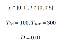
Since the wall has a 1 ft thickness, the problem space domain could be restricted between 0 and 1, and the diffusivity value, which is considered constant, could be set to 0.01. The time domain was restricted between 0 to 0.5:
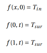
The initial boundaries can be formalized in mathematical expressions:
The analytical solution of this problem was given by the following expression
Numerical analysis is the study of the obtained solution. Criticism is very important on this phase, since the solutions are evaluated. Digital computers have problems with round-off errors, and since values were truncated, problems with discretization errors may appear. There are some definitions related with this study: stability, convergence and approximation.
A method is declared stable if the error doesn’t grow as time advances. Theoretically, conditions that make a scheme becomes stable or unstable can be known.
Approximation can be verified by comparing the computed solution with the analytical solution, and check if there is an approximation at all.
Convergence is defined by how well the computed solution approximates to the analytical solution. This can vary with a change in the number of time steps or space steps. A smaller number of steps can lead to a bigger error, whereas a bigger number of steps can lead to a considerably more time expensive solution. Every method could be developed using Taylor Series. This series were developed for n terms. Thus, every method has a given approximation factor, that could be represented in the Big Oh annotation. The error related with this approximation is called Truncation Error.
A quantitative analysis can be done by comparing solutions of each method. By calculating the norms of the error matrix, one can conclude which method is more accurate. The error matrix can be calculated by subtracting each cell of the analytical solution matrix to the cells of a method matrix. When the result is a matrix of small values, the error is small. Whenever a norm is calculated, one is able to translate an error matrix into a single value:
-
One Norm - Which is given by adding the absolute values of each cell of the matrix.
-
Two Norm - Which is obtained by adding the squares of every value in the matrix.
-
Uniform Norm - Which represents the biggest error, or the maximum value in the matrix.
The second norm “punishes” the biggest values, and “regards” the lowest ones. Notice that a the square of a value between 0 and 1 is lower than the given value. Whereas the square of a value bigger than 1 is higher. Therefore, this norm is a good quality indicator.
A stencil could also be developed for each method, which relates the several grid points, revealing the dependencies for a calculation in a more graphical way.
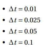
Four different schemes/methods were used to compute a solution for the given problem, two of them are explicit schemes, Richardson, DuFort-Frankel, and two of them are implicit schemes, Laasonen Simple Implicit and Crank-Nicholson. The space step was maintained at 0.05 ft, and the time step took the value of 0.01 h, studying every solutions in intervals of 0.1 hours from 0.0 to 0.5. The Laasonen Simple Implicit solution was also studied with different time steps, always maintaining the same space step, 0.05:
As referred, considering the initial equation, these methods can be written in its discretized form.
This type of schemes rely only on the previous time steps to calculate the current time step solution. In the case of both used methods, they were relying in known values of the n - 1 and n time steps to calculate a value for the n + 1 time step. Thereby, the second time step can not be calculated by these methods, because there’s no possible value for a negative time step. A different method, for the same equation, with two levels of time steps was used in order to overcome this situation, the Forward in Time and Central in Space scheme. It’s known that this method is conditionally stable, and its stability condition is given by,
Therefore, considering Delta t = 0.01, Delta x = 0.05, and D = 0.1, this method is declared stable. It’s important to have a stable solution for the first iteration, since it is a major influence on the overall solution. Therefore, this iteration could be calculated with the following expression,
 |
 |
|---|---|
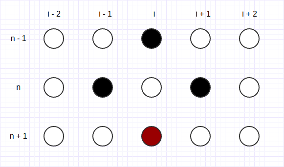
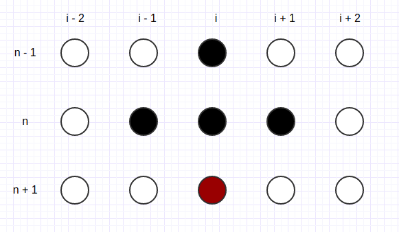
| Fig 1: Richardson stencil | Fig 2: Dufort-Frankel stencil |
The Richardson method can be applied by having a central in time and central in space scheme. Regarding to stability issues, this method is unconditionally unstable. Following the heat conduction equation, the expression could be represented at Figure 2 and could be written as following:
Which corresponds to,
The DuFort-Frankel scheme can be applied by having central differences
in both derivatives, but to prevent stability issues, the space
derivative term  can be written as the average value of
 and
and  . The method stencil can be observed
at Figure 1. Therefore this method is
declared as unconditionally stable and it may be formulated as follows:
Which is equivalent to,
In other hand, implicit schemes rely not only on lower time steps to calculate a solution, but also on the current time step known values. Each time step solution can often be solved by applying the Thomas Algorithm, which is an algorithm that can solve tridiagonal matrix systems, Ax = r. This algorithm is a special case of the LU decomposition, with a better performance. The matrix A can be decomposed in a lower triangular matrix L and an upper triangular matrix U, therefore A = LU$. This algorithm consists of two steps, the downwards phase where the equation Lp = r is solved and the upwards phase, solving Ux = p, obtaining a solution for x.
 |
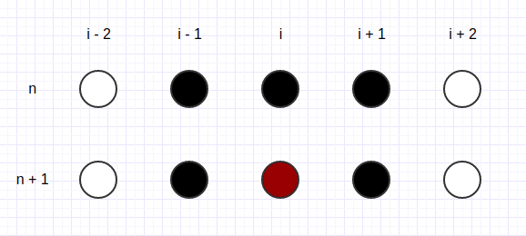 |
|---|---|
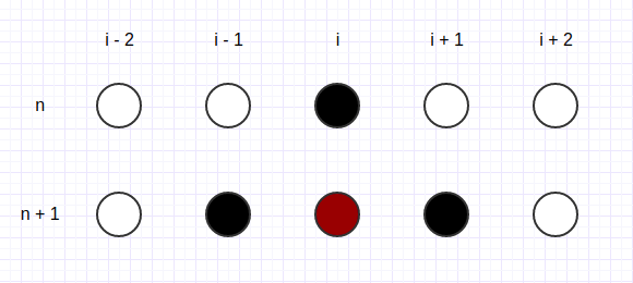
| Fig 3: Laasonen stencil | Fig 4: Crank-Nicholson stencil |
The time derivative is considered forward in time. Central difference is used in space derivative, and unconditionally stable. Concluding, the below equation could be established, and it could be represented at Figure 3:
Assuming that  , the equation could
be represented as:
The values of the first and last space position of each time step are known, they are represent by the TSur value. Therefore, in every second and penultimate space step, two terms of the previous equation could be successfully inquired. For the second space step, the equation could be divided by having the unknown terms in the left side and the known terms in the right side:
And the same could be done for the penultimate space step:
For every other space steps with unknown values, the expression could be generalized as:
Considering that the maximum number of space steps is m, the previous expressions could form a system of linear equations, A.x = r:
The time derivative is considered forward in time, and the space derivative can be replaced by the average of central differences in time steps n and n + 1. The method is declared unconditionally stable and it could be represented at Figure 4. Thus:
In this method, the coefficient had a new value,  , and assuming that
p is equal to the forward in space, central in time plus backwards in space, central in time derivatives, the equation could be written as follows,
Following the same logical principles of the previous scheme, some expressions could be generalized for the second,
, penultimate,
, and every other space steps with unknown values.
Thus, a tridiagonal matrix system is obtained,
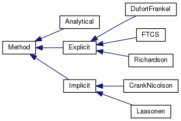
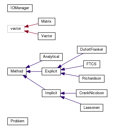
The code was first planned with an initial structure and suffered incremental upgrades. A method class was created, being a prototype with multiple inheritance, containing three sub classes: Analytical, Implicit and Explicit. Therefore, the Implicit class is an Abstract class as well. This class has three sub classes, representing the three explicit methods used in this problem. Similarly, the Implicit class is also an abstract class, having two implicit methods classes as sub classes. The previously described inheritance structure can be more easily visualized in the image below.
A Method class contains a Problem object. The Problem class represents the Heat Conduction problem, containing informations about the time and space steps, the solution and initial conditions.
An Input and Output Manager class was developed so that the code related with plots and tables exportations could be separated from the logical source code. This class was developed with several methods regarding data interpretation and structuration in order to easily export plot charts. A gnuplot C++ library was used, therefore the gnuplot syntax could be directly used from the c++ code, cutting down the need of developing external bash scripts for this specific purpose.
Despite the referred classes, a header file with useful macros was declared. This file contains information about which conditions to test, like the initial temperature and the surface temperature. Therefore, if for some reason, one of this values changes, it can be easily corrected.
The several objects in this structure could be instantiated in the main file, calling methods to compute the several solutions and to export their plot charts. The previously described classes can be represented in the following diagram.
The results of the four methods, Richardson, DuFort-Frankel, Laasonen Simple Implicit and Crank-Nicholson can be seen in the following figures/tables. These results were used to analyze each solution quantitatively and qualitatively. In most of the plot charts, the obtained solution was compared to the analytical solution so that it would be possible to realize whether the solution was a good approximation or not. Notice that the next results are regarding to the “default” values of time and space steps, time step = 0.01 and space step = 0.05.
| Table 2: Laasonen method error table |
|---|
 |
By examining Table 2, it could be concluded that the solution given by the Richardson method was considerably different from the analytical solution. This was due to the fact that this method is declared as unconditionally unstable. As referred before, when a method is declared unstable, the error grows as the time advances. The error growth was responsible for obtaining a different solution, or a solution to a different problem. The mathematical calculations regarding the stability and accuracy properties of this method can be found under the appendix section.
 |
|---|
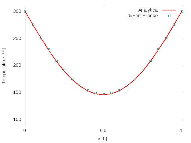
| Fig 7: DuFort-Frankel’s solution at t = 0.5. |
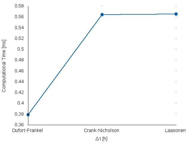
When looking at Figure 7, it can be observed that the DuFort-Frankel solution is quite approximated to the real solution. This scheme, as it could be observed at Figure 11, is more time efficient comparing to the implicit unconditionally stable methods, the only disadvantage is the fact that it requires a different method for the first iteration.
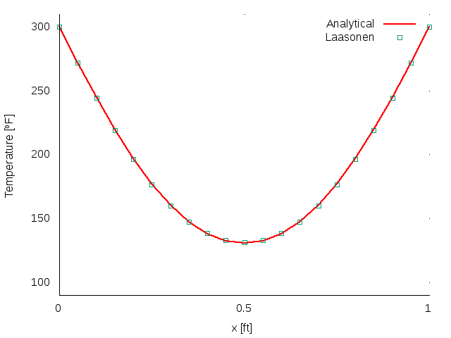
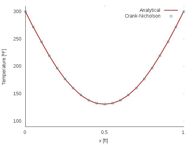
Similarly of what could be concluded on DuFort-Frankel results, by observing Figure 9 and Figure 8, it can also be deducted that these are good solutions. These schemes, Crank-Nicholson and Laasonen, are unconditionally stable as well. Therefore good results were expected.
 |
 |
|---|---|
| Fig 8: Laasonen’s solution at t = 0.4. | Fig 9: Crank-Nicholson’s solution at t = 0.4. |
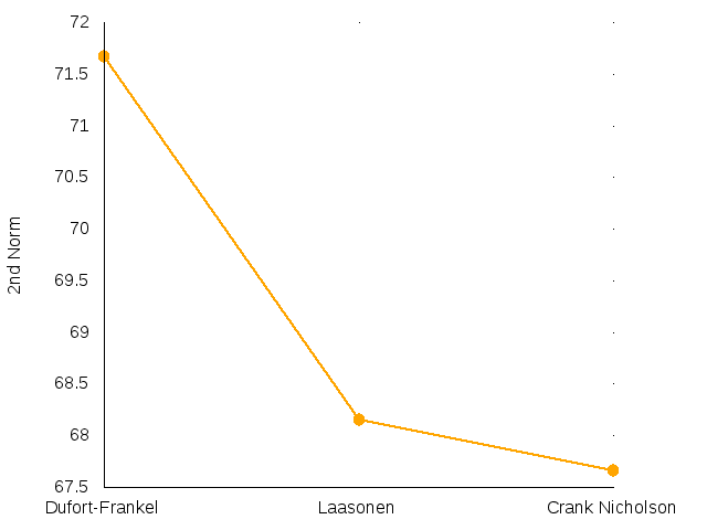
In other hand, when a quantitative analysis was done, it could be seen that the Crank Nicholson scheme is more accurate than the Laasonen and DuFort-Frankel methods. By looking at Figure 10, it can be observed that the second norm value of the Error matrix of this scheme is smaller than the values obtained by the other methods Error Matrices.
 |
 |
|---|---|
| Fig 10: 2nd norm values of Error Matrices. | Fig 11: Computational times of stable methods |
Laasonen Implicit Scheme is an unconditionally stable scheme to solve Parabolic Partial Differential Equations. Therefore, with the right time and space step, there’s almost no error related to the development of its results throughout the time advancement.
A reduction on these steps led to a higher computational time, since there’s more calculations to be made. Whereas steps with higher values led to more inaccurate results. This phenomenon could be explained with a concept that was introduced earlier, the truncation error. This error can only be avoided with exact calculations, but can be reduced by applying a larger number of smaller intervals or steps. As referred before, different results of this method were studied by changing the time step size. The space step was maintained at 0.05.
| Table 3: Laasonen method error table for the several time steps |
|---|
 |
Table 3 and figure 12 could support the previous affirmations. While observing table 3, it could be seen that the error is larger for bigger time steps, as it was expected. Whereas when observing figure 12, it can be identified a reduction in computational time as the time step becomes larger.
The obtained results could support the theoretical concepts. Unstable methods demonstrated an error growth through the time progress. The Forward in Time, Central in Space explicit scheme was stable with the given initial conditions, therefore it could support a good solution for the explicit stable scheme, DuFort-Frankel. As referred, the solution of the DuFort-Frankel method strongly depends on the first iteration solution.
It could be observed that smaller steps can lead to a time expensive solution, whereas larger steps lead to an error increase. Stable methods could give a good solution with the right time and space steps, but by analysing the second norm value, it was concluded that the Crank-Nicholson method is more accurate. This is due to the fact that this method has a better approximation order.
It is important to have a balance between the two problems (time and approximation), a method should be computed in an acceptable time, and still obtain a good result. In realistic scenarios the problem solution is not known, therefore error estimates are impractical. The used step size should be small as possible, as long as the solution is not dominated with round-off errors. The solution must be obtained with a number of steps that one has time to compute.

