priorsense

Overview

priorsense provides tools for prior diagnostics and sensitivity analysis.

It currently includes functions for performing power-scaling sensitivity analysis on Stan models. This is a way to check how sensitive a posterior is to perturbations of the prior and likelihood and diagnose the cause of sensitivity. For efficient computation, power-scaling sensitivity analysis relies on Pareto smoothed importance sampling (Vehtari et al., 2021) and importance weighted moment matching (Paananen et al., 2021).

Power-scaling sensitivity analysis and priorsense are described in Kallioinen et al. (2022).

Installation

Download the development version from GitHub with:

# install.packages("remotes")
remotes::install_github("n-kall/priorsense")

Usage

priorsense currently works with models created with rstan, cmdstanr or brms. However, moment matching currently does not work with cmdstan models.

Example

Consider a simple univariate model with unknown mu and sigma fit to some data y (available viaexample_powerscale_model("univariate_normal")):

data {
  int<lower=1> N;
  real y[N];
}
parameters {
  real mu;
  real<lower=0> sigma;
}
model {
  // priors
  target += normal_lpdf(mu | 0, 1);
  target += normal_lpdf(sigma | 0, 2.5);
  // likelihood
  target += normal_lpdf(y | mu, sigma);
}
generated quantities {
  vector[N] log_lik;
  // likelihood
  real log_prior;
  for (n in 1:N) log_lik[n] =  normal_lpdf(y[n] | mu, sigma);
  // joint prior specification
  log_prior = normal_lpdf(mu | 0, 1) +
    normal_lpdf(sigma | 0, 2.5);
}

We first fit the model using Stan:

library(priorsense)

normal_model <- example_powerscale_model("univariate_normal")

fit <- rstan::stan(
  model_code = normal_model$model_code,
  data = normal_model$data,
  refresh = FALSE,
  seed = 1234
)

Once fit, sensitivity can be checked as follows:

powerscale_sensitivity(fit)
#> Sensitivity based on cjs_dist:
#> # A tibble: 2 × 4
#>   variable prior likelihood diagnosis          
#>   <chr>    <dbl>      <dbl> <chr>              
#> 1 mu       0.368      0.519 prior-data conflict
#> 2 sigma    0.266      0.512 prior-data conflict

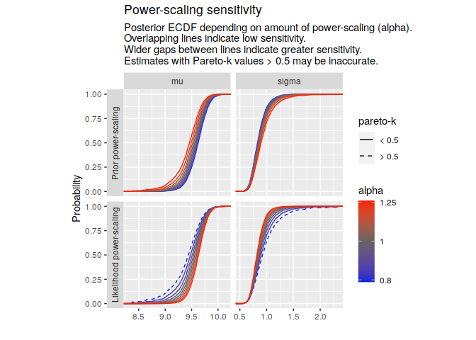
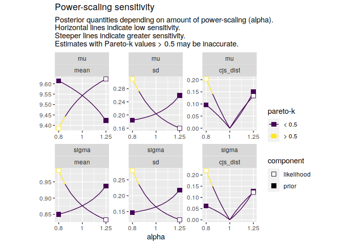
To visually inspect changes to the posterior, first create a power-scaling sequence.

pss <- powerscale_sequence(fit)
#> Warning: Some Pareto k diagnostic values are slightly high. See help('pareto-k-diagnostic') for details.

Then use a plotting function. Estimates that may be inaccurate (Pareto-k values > 0.5) are indicated.

powerscale_plot_ecdf(pss, variables = c("mu", "sigma"))

powerscale_plot_quantities(
  pss,
  quantities = c("mean", "sd"),
  div_measure = "cjs_dist",
  variables = c("mu", "sigma")
)

References

Noa Kallioinen, Topi Paananen, Paul-Christian Bürkner, Aki Vehtari (2022). Detecting and diagnosing prior and likelihood sensitivity with power-scaling. preprint arXiv:2107.14054

Topi Paananen, Juho Piironen, Paul-Christian Bürkner, Aki Vehtari (2021). Implicitly adaptive importance sampling. Statistics and Computing 31, 16. https://doi.org/10.1007/s11222-020-09982-2

Aki Vehtari, Daniel Simpson, Andrew Gelman, Yuling Yao, Jonah Gabry (2021). Pareto smoothed importance sampling. preprint arXiv:1507.02646

annariha / priorsense